Anti-DDoS research part 4: an information-gain oracle. Practical Python example

﷽

Hello, cybersecurity enthusiasts and white hackers!

In part 1 and part 2, I looked at wavelet-based traffic anomalies. In part 3, I used handshake asymmetry to detect SYN-flood campaigns.

Today the question is different: which question should a detector ask next?

We will build a small tree of questions about network flows, run it against the local CICDDoS2019 CSV files, and measure the trade-off between detection quality and the number of questions. The code and the measurements below use completed flow records. This is an offline classifier experiment, not a measurement of detection latency during a live flood.

idea - what is our oracle?

Call any yes/no probe that narrows down a set of hypotheses an oracle: it answers one question, and the algorithm keeps only the hypotheses consistent with that answer before asking the next one. This is adaptive hypothesis reduction, and it works the same whether the hypotheses are bits of a hidden state or, as here, traffic labels.

Our observation interface answers a question such as:

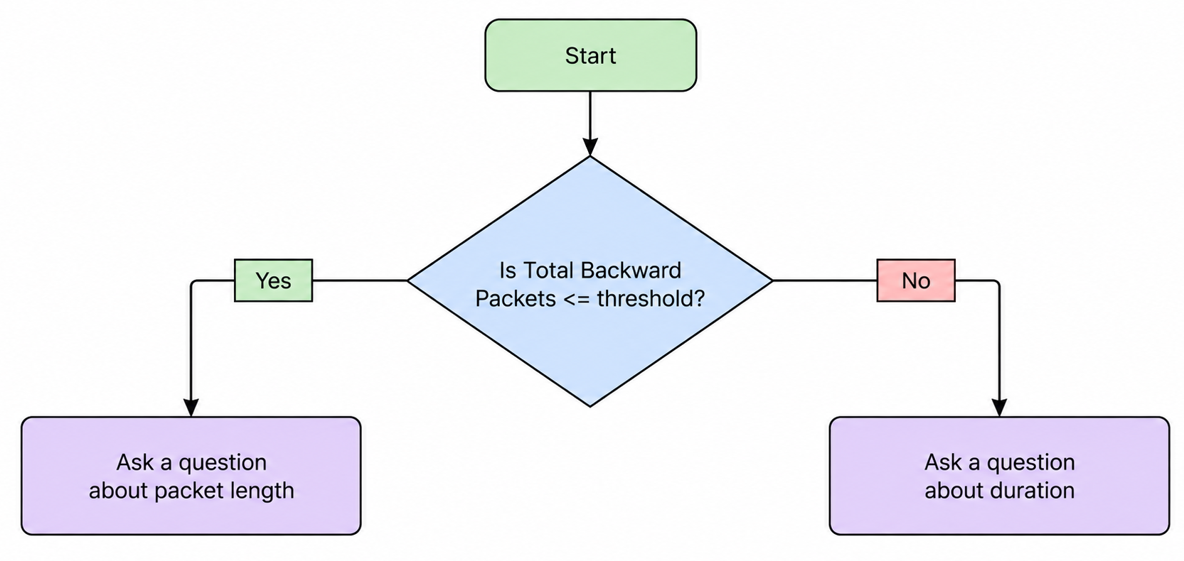
The thresholds and branches come from labelled training data. At inference time, the flow features answer the questions; the label is unavailable.

This construction is an entropy-based decision tree. Calling the observation interface an oracle does not make it a new classifier. The practical contribution is an auditable sequence of questions and an experiment with a question budget.

In plain english: a decision tree is a nested set of yes/no questions about a flow’s features, such as “is Total Length of Bwd Packets ≤ 85 bytes?”. Each answer routes the flow to one branch; once the tree runs out of allowed questions, or a branch is already pure enough, the leaf at the bottom reports a class. Building the tree means choosing, at every branch, the question that best separates benign from attack rows in the training data - which is exactly what the next two sections define precisely.

from candidate counts to information

Suppose an ideal noiseless oracle has N equally likely hypotheses, and a question divides them into two disjoint groups of sizes \(a\) and \(N-a\).

The expected number of surviving hypotheses is:

\[E[N_{\mathrm{next}}] = \frac{a}{N}a + \frac{N-a}{N}(N-a) = \frac{N}{2} + \frac{2}{N}\left(a-\frac{N}{2}\right)^2.\]

The square is nonnegative. Therefore a balanced split minimizes this expectation. For 100 candidates, a 50/50 split leaves 50 in expectation; a 90/10 split leaves 82.

This is an idealized, noiseless model: it assumes disjoint outcome groups and a uniform prior over hypotheses. Real probes are rarely that clean.

For traffic detection we care about the class, not the identity of a particular row. Splitting rows in half does not help if both halves have the same class mixture.

entropy - uncertainty about a label

Let \(Y\in\{0,1\}\), with 0 = BENIGN and 1 = non-BENIGN. At a tree node, let \(p\) be the fraction of attack-labelled training rows.

The uncertainty is:

\[h_2(p)=-p\log_2 p-(1-p)\log_2(1-p),\]

using \(0\log_2 0=0\) by continuity.

In plain english: \(h_2(p)\) measures how mixed the two classes are at a node. A node that is 100% attack or 100% benign has zero entropy - nothing left to guess. A 50/50 node has maximum entropy, 1 bit - a coin flip.

Its derivatives explain the shape:

\[h_2'(p)=\log_2\frac{1-p}{p}, \qquad h_2''(p)=-\frac{1}{\ln 2}\left(\frac{1}{p}+\frac{1}{1-p}\right)<0.\]

So entropy is concave, has its maximum of 1 bit at \(p=1/2\), and approaches zero at either pure class. Low entropy can mean “almost certainly benign” or “almost certainly attack”.

This is label entropy. Source-IP entropy measures a different random variable and cannot be substituted into this equation.

conditional information gain

A question is $Q_{j,t}(x)=\mathbf{1}[x_j\leq t]$. Here $j$ selects a feature and $t$ is a threshold. Let $S$ denote the observations on the path so far.

In plain english: a question is something like “is Total Length of Bwd Packets ≤ 85?” - every row answers yes or no, and the two answers become the tree’s two branches.

The expected reduction in uncertainty is:

\[I(Y;Q\mid S) =H(Y\mid S) -\sum_{b\in\{0,1\}}P(Q=b\mid S)H(Y\mid S,Q=b).\]

At a training node containing $n$ rows, this becomes:

\[IG=h_2(p)-\frac{n_L}{n}h_2(p_L)-\frac{n_R}{n}h_2(p_R).\]

In plain english: IG is how much the entropy drops, on average, once we know the answer. A good question sends most attack rows one way and most benign rows the other, pushing both children toward purity and toward zero entropy.

We choose the admissible feature and threshold with the greatest gain, then repeat inside each child node. Reusing an unconditional feature ranking at every step misses the conditioning on earlier answers.

For example, start with 50 benign + 50 attack rows. A candidate question creates:

Branch	Benign	Attack	Attack fraction
left	40	10	0.2
right	10	40	0.8

The gain is:

\[IG=1-\frac12h_2(0.2)-\frac12h_2(0.8) =1-0.721928 =0.278072\ \mathrm{bits}.\]

A question producing 25 benign + 25 attack in both branches also splits rows evenly, but its gain is zero. Splitting the rows evenly is not the same as splitting the classes: both branches still look exactly like the original 50/50 mix, so the question told us nothing new about the label.

At inference, the empirical leaf fraction estimates \(P(Y=1\mid S)\). Bayes’ rule describes an update conceptually:

\[P(Y=y\mid S,Q=b) =\frac{P(Q=b\mid Y=y,S)P(Y=y\mid S)} {\sum_c P(Q=b\mid Y=c,S)P(Y=c\mid S)}.\]

In plain english: once we know the answer to a question, we update our belief about the label using how likely that answer was under each class - the same logic as updating a diagnosis after a medical test result.

The tree estimates conditional mixtures directly from training subsets; we do not multiply marginal feature likelihoods as though packet counts and byte counts were independent.

Entropy-based splitting and leaf class fractions are standard decision-tree mechanics; see the scikit-learn tree documentation.

dataset - use what the files actually contain

I use the local dir with previous dataset here:

tree ./03-11

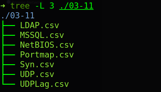
It contains LDAP.csv, MSSQL.csv, NetBIOS.csv, Portmap.csv, Syn.csv, UDP.csv, and UDPLag.csv. Each inspected header has 88 columns, including Label. Headers have leading spaces, which the loader strips.

The source is CICDDoS2019, Canadian Institute for Cybersecurity. The experiment below is a custom cross-file evaluation of this local subset, not the official training-day/testing-day benchmark.

Do not infer labels from filenames: the full label inventory printed by the program shows that a file can contain several attack labels as well as benign flows.

Our binary target uses the actual Label field. This experiment does not claim to distinguish an HTTP flood, and these flow counters do not directly provide HTTP request rates or completed TCP handshake counts.

The selected inputs are:

CSV feature	What this experiment observes
Flow Duration	Recorded duration of a flow
Total Fwd Packets / Total Backward Packets	Directional packet counts
Total Length of Fwd Packets / Total Length of Bwd Packets	Directional byte totals
SYN Flag Count / ACK Flag Count	Exported flag-count features
Packet Length Mean	Exported mean packet length

In particular, an ACK counter is not a count of completed three-way handshakes. Source entropy would require grouping multiple flows into windows; a single row is insufficient.

practical example - bounded memory and an honest split

Loading all 88 columns from every CSV and concatenating them wastes memory. The script reads only the eight features and label, in chunks of 100000 rows.

Each row receives an independent uniform random priority. Keeping the smallest 12000 priorities per file gives a uniform sample without replacement from the entire file, rather than its first few minutes. A fixed seed makes the sample reproducible. Memory scales with the chunk size and retained samples, not the combined CSV size.

This is the standard reservoir-sampling trick: since every row’s priority is drawn independently and uniformly, keeping the k smallest priorities is equivalent to a uniform random subset of size k, regardless of file order or size.

The program performs seven folds. Each time, one file supplies test rows and the other six supply training rows. It fits imputation medians and all tree thresholds on training rows only. IPs, ports, Flow ID, timestamp, filename, Inbound, and SimillarHTTP are excluded from the feature matrix.

This avoids direct file-identifier learning and random row splitting within one file. It does not prove independence between captures: hosts, generator patterns, or duplicated flows may still overlap across files. No cross-file deduplication is performed. Treat the results as cross-file transfer measurements, not proof of production or unseen-day performance.

For each fold we compare a majority-class baseline with tree depths 1, 2, 4, 8. Each tree has at least 100 training rows per leaf. That is a fixed regularizer for this experiment, not a tuned optimum.

practical example - code

The complete runnable source is included here (oracle.py):

#!/usr/bin/env python3
"""Offline CICDDoS2019 experiment; uniformly sample each complete CSV."""
import argparse
import json
from pathlib import Path

import numpy as np
import pandas as pd
from sklearn.tree import DecisionTreeClassifier, export_text

FEATURES = ["Flow Duration", "Total Fwd Packets", "Total Backward Packets",
            "Total Length of Fwd Packets", "Total Length of Bwd Packets",
            "SYN Flag Count", "ACK Flag Count", "Packet Length Mean"]


def sample_file(path, cap, seed):
    rng = np.random.default_rng(seed)
    kept = pd.DataFrame()
    counts = {}
    scanned = 0
    for chunk in pd.read_csv(path, usecols=lambda c: c.strip() in FEATURES + ["Label"],
                             chunksize=100000, low_memory=False):
        chunk.columns = chunk.columns.str.strip()
        labels = chunk["Label"].astype("string").str.strip()
        for label, n in labels.fillna("<missing>").value_counts().items():
            counts[str(label)] = counts.get(str(label), 0) + int(n)
        scanned += len(chunk)
        valid = labels.notna() & labels.ne("")
        chunk = chunk.loc[valid].copy()
        chunk["Label"] = labels.loc[valid]
        chunk["priority"] = rng.random(len(chunk))
        kept = pd.concat([kept, chunk], ignore_index=True).nsmallest(cap, "priority")
    if kept.empty:
        raise ValueError(f"No labelled rows: {path}")
    x = kept[FEATURES].apply(pd.to_numeric, errors="coerce").to_numpy(dtype=float)
    x[~np.isfinite(x)] = np.nan
    y = kept["Label"].str.upper().ne("BENIGN").to_numpy(dtype=int)
    return x, y, {"file": path.name, "scanned": scanned, "labels": counts,
                  "sample": len(y), "sample_benign": int((y == 0).sum())}


def rate(a, b):
    return float(a / b) if b else None


def main():
    parser = argparse.ArgumentParser()
    parser.add_argument("data", type=Path)
    parser.add_argument("--cap", type=int, default=12000)
    parser.add_argument("--seed", type=int, default=7)
    parser.add_argument("--output", type=Path, default=Path("oracle-results.json"))
    args = parser.parse_args()
    if args.cap < 1:
        parser.error("--cap must be positive")
    files = sorted(args.data.glob("*.csv"))
    if len(files) < 2:
        parser.error("Need at least two CSV files")
    samples = []
    inventory = []
    for i, path in enumerate(files):
        x, y, info = sample_file(path, args.cap, args.seed + i)
        samples.append((x, y))
        inventory.append(info)
        print(json.dumps(info), flush=True)
    results = []
    for held, path in enumerate(files):
        train_x = np.concatenate([s[0] for i, s in enumerate(samples) if i != held])
        train_y = np.concatenate([s[1] for i, s in enumerate(samples) if i != held])
        if len(np.unique(train_y)) != 2:
            raise ValueError("Training fold needs both benign and attack rows")
        # Train-only imputation; no global quantiles or identifiers.
        medians = np.nanmedian(train_x, axis=0)
        medians = np.nan_to_num(medians, nan=0.0)
        train_x = np.where(np.isnan(train_x), medians, train_x)
        test_x, test_y = samples[held]
        test_x = np.where(np.isnan(test_x), medians, test_x)
        for depth in [0, 1, 2, 4, 8]:
            if depth == 0:
                pred = np.full(len(test_y), int(train_y.mean() >= 0.5))
                questions = np.zeros(len(test_y))
            else:
                model = DecisionTreeClassifier(criterion="entropy", max_depth=depth,
                                               min_samples_leaf=100, random_state=args.seed)
                model.fit(train_x, train_y)
                pred = model.predict(test_x)
                questions = np.diff(model.decision_path(test_x).indptr) - 1
                if held == 0 and depth == 2:
                    print(export_text(model, feature_names=FEATURES), flush=True)
            tn = int(((test_y == 0) & (pred == 0)).sum())
            fp = int(((test_y == 0) & (pred == 1)).sum())
            fn = int(((test_y == 1) & (pred == 0)).sum())
            tp = int(((test_y == 1) & (pred == 1)).sum())
            results.append(dict(file=path.name, depth=depth, tn=tn, fp=fp, fn=fn, tp=tp,
                                fpr=rate(fp, fp + tn), recall=rate(tp, tp + fn),
                                precision=rate(tp, tp + fp),
                                mean_questions=float(questions.mean())))
    args.output.write_text(json.dumps({"seed": args.seed, "cap": args.cap,
                                      "features": FEATURES, "inventory": inventory,
                                      "results": results}, indent=2) + "\n")
    for depth in [0, 1, 2, 4, 8]:
        rows = [r for r in results if r["depth"] == depth]
        counts = {k: sum(r[k] for r in rows) for k in ["tn", "fp", "fn", "tp"]}
        print(json.dumps(dict(depth=depth, **counts,
                              fpr=rate(counts["fp"], counts["fp"] + counts["tn"]),
                              recall=rate(counts["tp"], counts["tp"] + counts["fn"]))))


if __name__ == "__main__":
    main()

Create an environment and run:

python3 -m venv venv
source ./venv/bin/activate
python -m pip install numpy==2.2.4 pandas==3.0.2 scikit-learn==1.9.0
python oracle.py ./03-11 --cap 12000 --seed 7 --output oracle-results.json

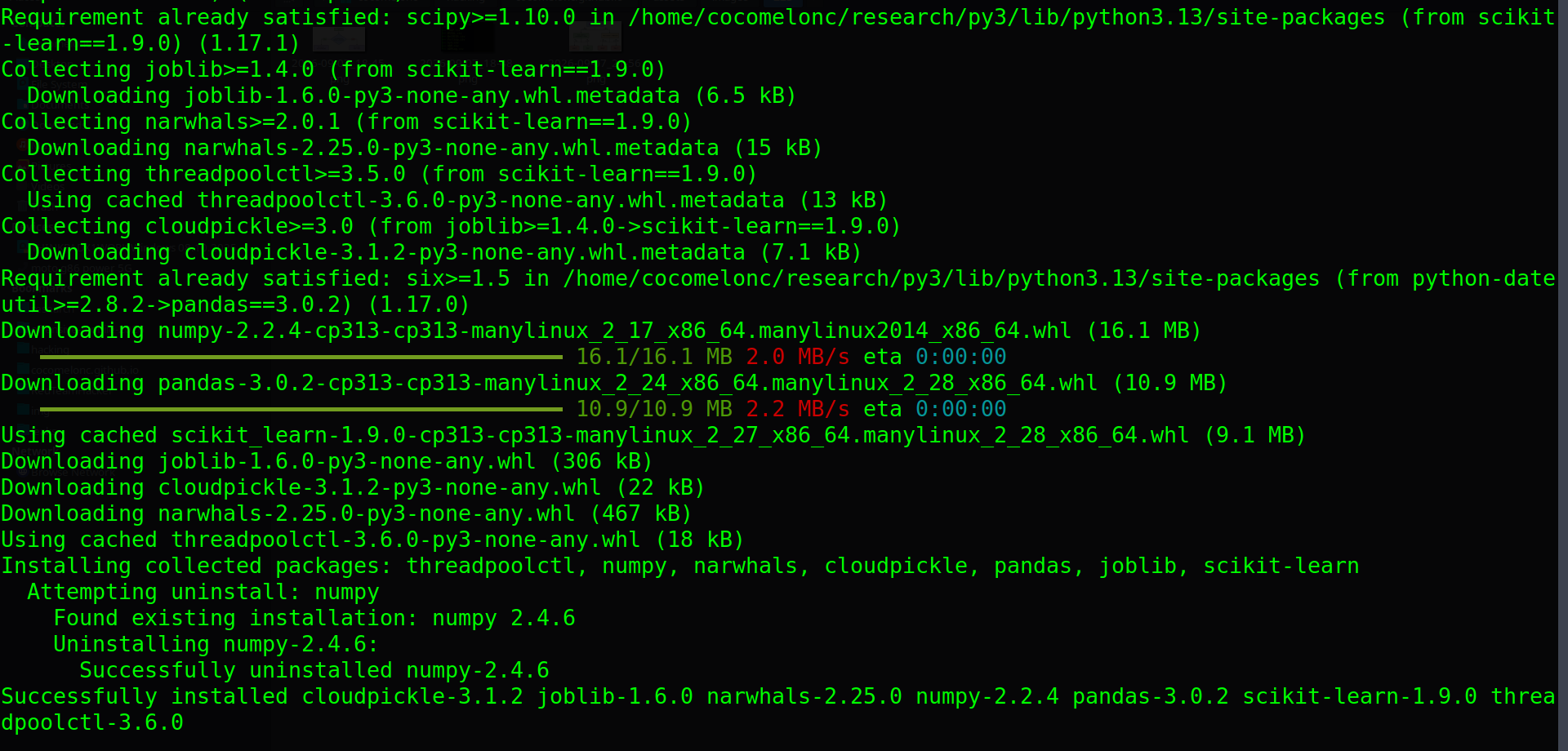
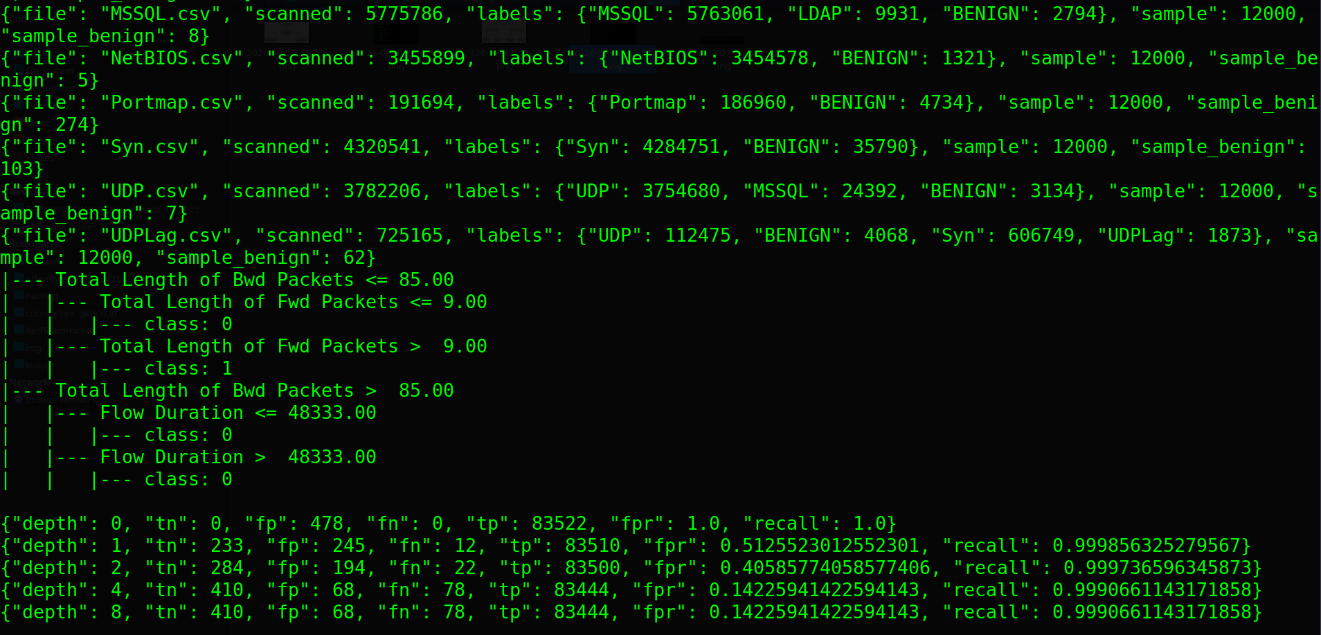
These are the library versions used for the recorded run. The script scans every selected CSV even with a small --cap; this option limits retained rows, not disk I/O. It prints the full label inventory before fitting models.

The printed depth-two tree shows the learned questions for the first held-out file. It is useful to inspect the actual thresholds instead of imagining that the tree necessarily learns a SYN/ACK test.

practical example - measured results

The recorded run scanned 20,364,525 rows and retained 84,000: 478 benign and 83,522 attack-labelled flows. Every retained row is tested once, in its held-out file’s fold. The baseline therefore has about 99.43% accuracy while misclassifying every benign flow.

Maximum depth	TN	FP	FN	TP	FPR	Recall	Mean questions
0	0	478	0	83522	100.00%	100.000%	0.00
1	233	245	12	83510	51.26%	99.986%	1.00
2	284	194	22	83500	40.59%	99.974%	2.00
4	410	68	78	83444	14.23%	99.907%	3.85
8	410	68	78	83444	14.23%	99.907%	5.48

Increasing depth from 2 to 4 reduces false positives from 194 to 68, at the expense of additional missed attack flows. Depth 8 produces the same pooled confusion counts in this run. A 14.23% benign false-positive rate is not a deployable blocking rule, despite recall above 99.9%.

At depth 4, the held-out files reveal the variation:

Held-out file	Sampled benign	False positives	Missed attack flows
LDAP.csv	19	0	11
MSSQL.csv	8	0	1
NetBIOS.csv	5	0	37
Portmap.csv	274	20	11
Syn.csv	103	26	15
UDP.csv	7	0	0
UDPLag.csv	62	22	3

Here is the actual depth-two tree with LDAP.csv held out. Class 0 is benign; class 1 is attack:

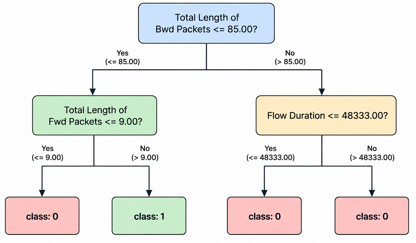
Both duration branches predict benign, yet their class mixtures can differ: entropy gain need not change the majority label. This also illustrates why information gain and decision utility are not identical.

The full recorded inventory and fold results are saved as oracle-results.json alongside the script in the source repository.

The output JSON preserves every held-out file’s confusion counts and mean path length, so pooled numbers need not hide a weak fold.

We count questions as internal nodes visited:

\[q(x)=|\mathrm{decision\_path}(x)|-1.\]

The subtraction removes the terminal leaf. A depth-d tree asks at most d questions, but may stop earlier. The same feature can appear twice along a path, so this count is not the number of distinct features acquired.

All features were already exported to CSV. We measure comparisons, not packet-capture cost, CPU savings in a live sensor, or end-to-end mitigation latency.

why accuracy alone is misleading

With attacks dominating the sample, “always attack” can have impressive accuracy and still reject every benign flow.

The metrics are:

\[FPR=\frac{FP}{FP+TN}, \qquad TPR=\frac{TP}{TP+FN}, \qquad \mathrm{precision}=\frac{TP}{TP+FP}.\]

Undefined rates are serialized as null, not zero. Equal per-file sample caps change the pooled file mixture, so pooled metrics describe our sampling protocol rather than the volume-weighted original collection.

Base rates matter too. If deployment attack prevalence is \(\pi\), then:

\[P(\mathrm{attack}\mid\mathrm{alert}) =\frac{TPR\,\pi}{TPR\,\pi+FPR(1-\pi)}.\]

As a numerical example, TPR = 0.99, FPR = 0.01, and \(\pi=0.001\) give only about 9.0% attack probability among alerts. Those are illustrative numbers, not measurements from this run. This is the base-rate fallacy: when attacks are rare events, most alerts still come from the much larger pool of benign flows, even at a low false-positive rate.

Few benign samples also mean uncertain FPR estimates. With zero false positives in \(n\) independent benign trials, the one-sided 95% binomial upper bound is:

\[FPR_{\mathrm{upper}}=1-0.05^{1/n}\approx\frac{3}{n}.\]

At n = 100, zero observed false positives is compatible with an FPR near 3%. Correlated flow records weaken the independent-trial assumption further.

a deeper extension - information has a price

For an actual sensor, different observations have different costs. A candidate objective is:

\[Q^\star=\arg\max_Q\left[I(Y;Q\mid S)-\lambda c(Q,S)\right].\]

In plain english: prefer a question that reveals a lot per unit of cost. A cheap check on an already-computed counter can beat an expensive one that requires waiting for more packets, even if the expensive one reveals slightly more.

Here \(c\) may represent computation or collection delay, and \(\lambda\) converts that cost into the same scale as information. Re-reading a cached counter may be cheap; waiting for a flow to finish may dominate the cost. Our code uses ordinary entropy gain and a depth limit; it does not implement this cost-sensitive extension.

Even maximum information gain is not the same as minimum decision loss. Let a false alert cost \(C_{FP}\) and a missed attack cost \(C_{FN}\). If \(p=P(Y=1\mid S)\) is calibrated, alerting is cheaper when:

\[C_{FP}(1-p)<C_{FN}p \quad\Longleftrightarrow\quad p>\frac{C_{FP}}{C_{FP}+C_{FN}}.\]

Leaf fractions are not automatically calibrated deployment probabilities. Select operating thresholds and check calibration on separate representative validation data.

A one-step value-of-information rule would ask another question only when its expected reduction in decision loss exceeds its cost:

\[R(p)=\min\{C_{FN}p,\ C_{FP}(1-p)\},\]

In plain english: \(R(p)\) is the cost of the cheaper mistake - guess “attack” and risk a false alarm, or guess “benign” and risk missing a real attack - whichever guess costs less on average given the current belief \(p\).

\[R(p)-\sum_b P(Q=b\mid S)R(p_b)>c(Q,S),\]

where cost is now measured in decision-loss units. This equation explains why a detector may stop even while some entropy remains: another observation may not change the appropriate action.

practical example - plotting the trade-off

The tables above are exact, but a plot makes the trade-off easier to read at a glance. oracle.py already saved every fold’s confusion counts and mean question count into oracle-results.json, so plotting is a separate, small script that only reads that JSON - no need to touch the CSVs again.

Here is plot_oracle.py:

#!/usr/bin/env python3
"""Plot the pooled question-budget/quality trade-off and per-file errors
from oracle-results.json (produced by oracle.py)."""
import json
from collections import defaultdict

import matplotlib.pyplot as plt


def load(path):
    with open(path) as f:
        return json.load(f)


def pooled_by_depth(results):
    agg = defaultdict(lambda: dict(tn=0, fp=0, fn=0, tp=0, q_sum=0.0, n=0))
    for r in results:
        d = agg[r["depth"]]
        for k in ("tn", "fp", "fn", "tp"):
            d[k] += r[k]
        n = r["tn"] + r["fp"] + r["fn"] + r["tp"]
        d["q_sum"] += r["mean_questions"] * n
        d["n"] += n
    rows = []
    for depth, d in sorted(agg.items()):
        fpr = d["fp"] / (d["fp"] + d["tn"])
        recall = d["tp"] / (d["tp"] + d["fn"])
        mean_q = d["q_sum"] / d["n"]
        rows.append((depth, mean_q, fpr, recall))
    return rows


def plot_tradeoff(rows, out):
    depths = [r[0] for r in rows]
    mean_q = [r[1] for r in rows]
    fpr = [r[2] * 100 for r in rows]
    recall = [r[3] * 100 for r in rows]

    fig, ax1 = plt.subplots(figsize=(8, 5))
    ax1.plot(mean_q, fpr, "o-", color="#d62728", linewidth=1.8, label="FPR")
    ax1.set_xlabel("mean questions asked per flow")
    ax1.set_ylabel("FPR, %", color="#d62728")
    ax1.tick_params(axis="y", labelcolor="#d62728")
    for x, y, d in zip(mean_q, fpr, depths):
        ax1.annotate(f"depth {d}", (x, y), textcoords="offset points", xytext=(8, 8))

    ax2 = ax1.twinx()
    ax2.plot(mean_q, recall, "s-", color="#2ca02c", linewidth=1.8, label="Recall")
    ax2.set_ylabel("Recall, %", color="#2ca02c")
    ax2.tick_params(axis="y", labelcolor="#2ca02c")
    ax2.set_ylim(99.5, 100.05)

    ax1.set_title("Question budget vs. detection quality (pooled, 7 folds)")
    ax1.grid(True, alpha=0.25)
    fig.tight_layout()
    fig.savefig(out, dpi=160)
    print(f"wrote {out}")


def plot_per_file(results, out, depth=4):
    rows = [r for r in results if r["depth"] == depth]
    rows.sort(key=lambda r: r["file"])
    files = [r["file"] for r in rows]
    fp = [r["fp"] for r in rows]
    fn = [r["fn"] for r in rows]

    x = range(len(files))
    width = 0.35
    fig, ax = plt.subplots(figsize=(9, 5))
    ax.bar([i - width / 2 for i in x], fp, width,
           label="false positives (benign flagged as attack)", color="#d62728")
    ax.bar([i + width / 2 for i in x], fn, width,
           label="missed attacks", color="#1f77b4")
    ax.set_xticks(list(x))
    ax.set_xticklabels(files, rotation=30, ha="right")
    ax.set_ylabel("flows")
    ax.set_title(f"Per-file errors at depth {depth} (held-out fold)")
    ax.legend()
    ax.grid(True, alpha=0.25, axis="y")
    fig.tight_layout()
    fig.savefig(out, dpi=160)
    print(f"wrote {out}")


def main():
    data = load("oracle-results.json")
    rows = pooled_by_depth(data["results"])
    for depth, mean_q, fpr, recall in rows:
        print(f"depth={depth} mean_questions={mean_q:.2f} fpr={fpr:.4f} recall={recall:.5f}")
    plot_tradeoff(rows, "oracle_depth_tradeoff.png")
    plot_per_file(data["results"], "oracle_per_file_depth4.png")


if __name__ == "__main__":
    main()

Run it against the JSON produced earlier:

python3 -m pip install matplotlib==3.10.9
python3 plot_oracle.py

In my case:

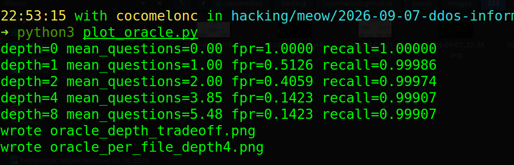
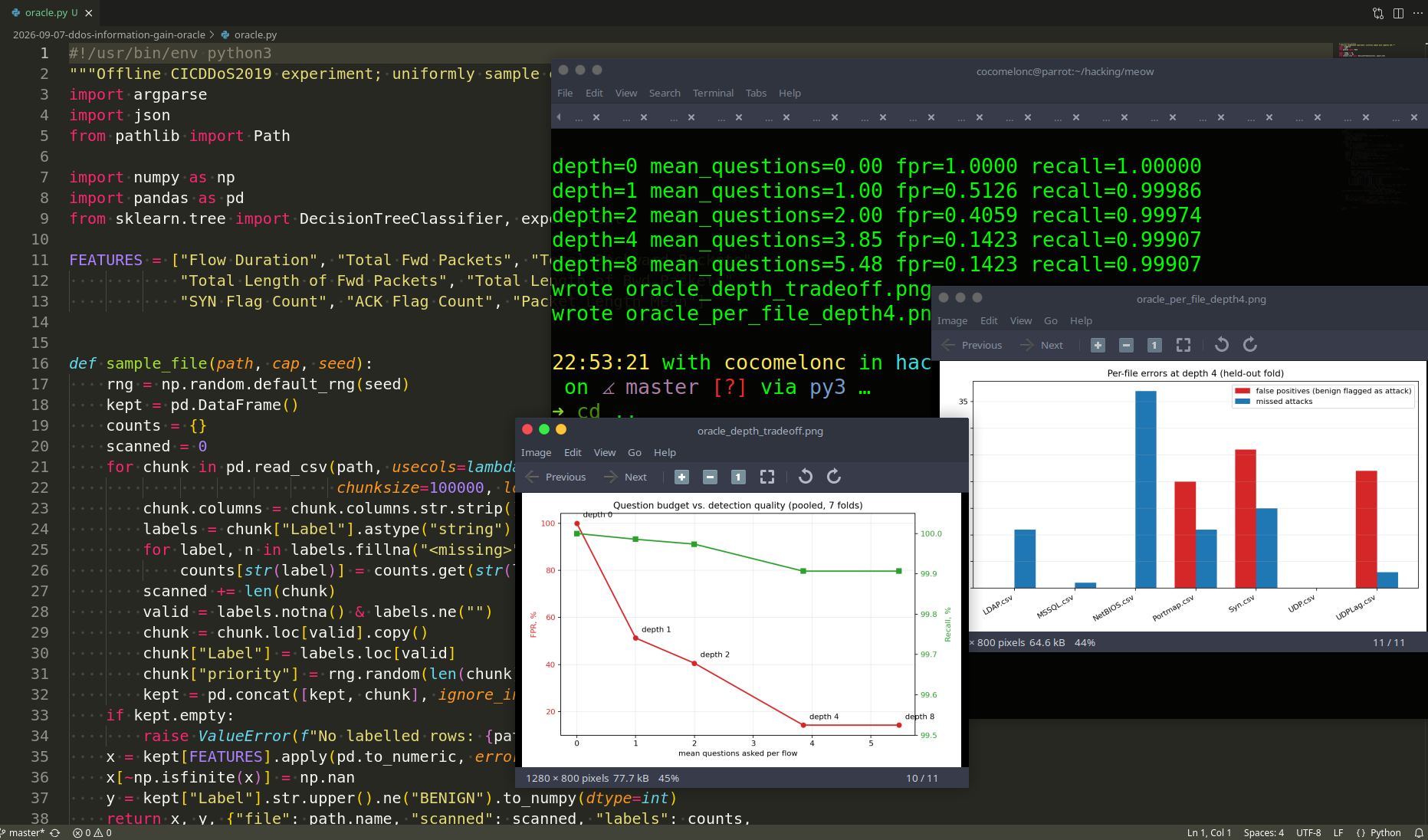
These numbers are exactly the pooled table from the previous section, only recomputed from the same JSON. First, the trade-off curve:

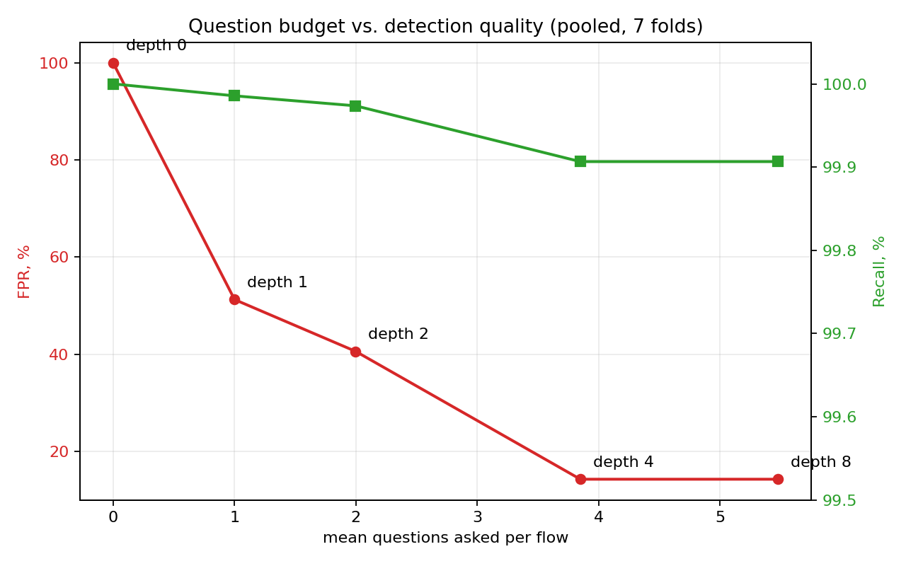
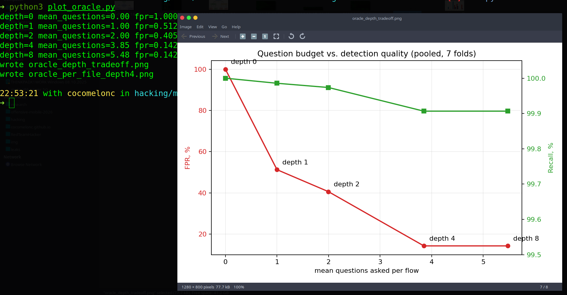
FPR falls steeply from depth 0 to depth 4, while recall barely moves off 100%. Depth 8 sits on top of depth 4: it asks more questions on average but buys nothing in this run, which is the diminishing-returns picture the question-budget framing predicts.

Second, where the depth-4 errors actually live:

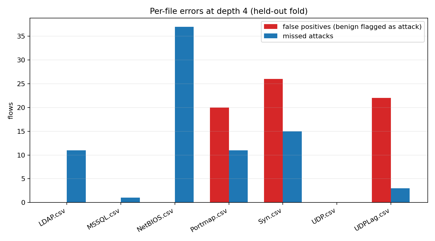
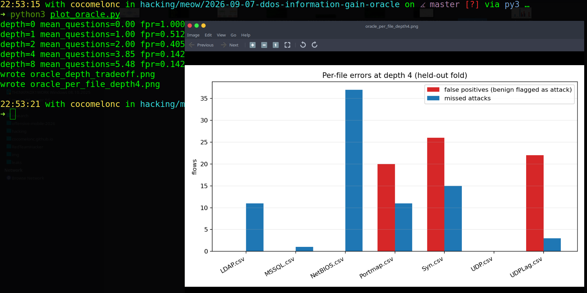
The pooled row hides that FPR is not evenly distributed: LDAP.csv, MSSQL.csv, and UDP.csv contribute zero false positives, while Portmap.csv, Syn.csv, and UDPLag.csv do all of the false-alarming. Missed attacks are just as lopsided in the other direction: NetBIOS.csv alone accounts for 37 of the 78 pooled false negatives. A single pooled FPR/recall number would have hidden both of these facts.

discussion

The concrete result is a reproducible flow-classification experiment with a visible path of questions, a majority baseline, and a question-budget comparison. It does not establish that a particular live endpoint is under DDoS, or that a completed-flow classifier can intervene before a service is affected.

A natural continuation of part 3 is to aggregate these observations into timestamped destination windows and evaluate campaign detection delay and false alerts per hour. That requires a new experiment: flow-level TPR cannot be relabelled as campaign recall.

The oracle framing helped us ask a useful question: which question should the detector ask next? The mathematics then made its limits clear: balanced candidate partitions, conditional label information, and operational decision costs are related but distinct objectives. The plots make the same point visually: FPR and mean questions both flatten out past depth 4, and the pooled numbers hide which file each error actually came from.

One more angle, since this whole post is really about spending a question budget efficiently: the same structure shows up on the other side of the fence. Sandbox-aware malware treats its execution environment as an oracle too - it asks cheap questions (CPU core count, uptime, screen resolution, recent mouse movement, specific registry or file artifacts) and only commits to malicious behavior once its hypothesis “this is a real host, not an analysis sandbox” has collapsed to high confidence. That is the same \(Q^\star=\arg\max_Q[I(Y;Q\mid S)-\lambda c(Q,S)]\) from the cost-aware section above, just with \(Y\) flipped to “real host vs. sandbox” and \(Q\) drawn from environment artifacts instead of flow features. The defensive implication is symmetric to the DDoS case: a sandbox should avoid letting any single cheap probe answer with a clean, high-information signal - the same reason we would not want one flow feature alone to leak the whole label.

DDoS2019 dataset and publication information

Dataset reference: Iman Sharafaldin, Arash Habibi Lashkari, Saqib Hakak, and Ali A. Ghorbani, “Developing Realistic Distributed Denial of Service (DDoS) Attack Dataset and Taxonomy,” IEEE ICCST, 2019.

source code in github

This is a practical defensive case for educational purposes only.

Thanks for your time happy hacking and good bye! PS. All drawings and screenshots are mine