Anti-DDoS research part 2: Daubechies D4 wavelet for traffic anomaly detection. Simple C example.

﷽

Hello, cybersecurity enthusiasts and white hackers!

In the previous post I started with the simplest possible wavelet: Haar. Haar is great for explaining the core idea: short traffic pulses can be invisible to rolling averages, but visible to wavelet detail coefficients.

Today I want to make the idea a little bit more serious. We will replace Haar with the Daubechies D4 wavelet. It is still small enough to implement in plain C, but mathematically it is more interesting because it has more structure and better behavior on smooth traffic trends.

Just defensive signal processing on traffic time series.

idea

Suppose we have a traffic feature:

flows per second
packets per second
SYN packets per second
DNS queries per second
sum of Total Fwd Packets from CICFlowMeter rows

For this post, the detector expects a simple CSV:

t,value,label
0,120.0,0
1,122.0,0
...
170,1450.0,1

where:

t is time bucket;
value is aggregated traffic feature;
label=0 means benign;
label=1 means attack.

This is a good format for public datasets such as CICDDoS2019, because CICDDoS2019 provides CICFlowMeter CSV files with timestamps and labels.

The official CIC page says that CICDDoS2019 contains benign traffic and modern DDoS attacks, includes true real-world-like PCAPs, and also includes CICFlowMeter-V3 CSV files with more than 80 traffic features and labels based on timestamp, IPs, ports, protocols and attack. Source: https://www.unb.ca/cic/datasets/ddos-2019.html

why not only rolling average?

A rolling average detector does this:

\[\bar{x}_t=\frac{1}{W}\sum_{i=0}^{W-1}x_{t-i}\]

and alerts when:

\[\bar{x}_t>\theta\]

This works for long attacks. But it has two problems:

short attacks can be averaged away;
after a short attack ends, the average can stay high and create a post-attack alert tail.

The second problem is important. In production systems this can lead to bad mitigation TTLs, slow recovery, and unnecessary blocking after the traffic has already normalized.

Daubechies D4

The Daubechies D4 wavelet uses four low-pass coefficients:

\[h_0=\frac{1+\sqrt{3}}{4\sqrt{2}}\] \[h_1=\frac{3+\sqrt{3}}{4\sqrt{2}}\] \[h_2=\frac{3-\sqrt{3}}{4\sqrt{2}}\] \[h_3=\frac{1-\sqrt{3}}{4\sqrt{2}}\]

Numerically:

h0 =  0.4829629131
h1 =  0.8365163037
h2 =  0.2241438680
h3 = -0.1294095226

from this low-pass filter we build the high-pass detail filter:

\[g_k=(-1)^k h_{3-k}\]

So:

\[g_0=h_3,\quad g_1=-h_2,\quad g_2=h_1,\quad g_3=-h_0\]

The streaming detail coefficient used in this PoC is:

\[d_t = g_0x_{t-3}+g_1x_{t-2}+g_2x_{t-1}+g_3x_t\]

Then we use absolute detail energy:

\[e_t=|d_t|\]

And a robust z-score:

\[z_t=\frac{e_t-\operatorname{median}(E_{baseline})} {1.4826\cdot\operatorname{MAD}(E_{baseline})}\]

where:

\[\operatorname{MAD}(E)= \operatorname{median}(|E_i-\operatorname{median}(E)|)\]

finally:

\[\text{alert}_t = \begin{cases} 1, & z_t>\tau \\ 0, & z_t\le\tau \end{cases}\]

why D4 is better than Haar in this case

Haar has two coefficients. D4 has four. This gives D4 a very useful property: two vanishing moments.

For the high-pass filter:

\[\sum_{k=0}^{3}g_k=0\]

and:

\[\sum_{k=0}^{3}k g_k=0\]

What does this mean in simple words?

If traffic is almost constant:

\[x_t=a\]

then:

\[d_t=0\]

If traffic is a smooth linear trend:

\[x_t=a+bt\]

then D4 still suppresses it much better than a simple edge detector.

but if traffic suddenly jumps:

\[x_t = \begin{cases} B, & t<t_0 \\ A, & t\ge t_0 \end{cases}\]

then:

\[d_t \neq 0\]

near the jump.

this is exactly what we want for short DDoS bursts: ignore smooth baseline movement, react strongly to abrupt changes.

practical example

for local reproducibility, I created a small CICDDoS2019-style time series:

baseline traffic around 120;
attack event 1 around t=170..176;
attack event 2 around t=260..268;
labels use 0 for benign and 1 for attack.

this fixture is not the full CICDDoS2019 dataset. It is a tiny local sample in the same time-series format. The included converter script can turn real CICDDoS2019 flow CSV into this format.

first, create the local fixture:

#!/usr/bin/env python3
import csv
import math


def is_attack(t):
    return 170 <= t <= 176 or 260 <= t <= 268


def value_at(t):
    baseline = 120.0 + 16.0 * math.sin(2.0 * math.pi * t / 96.0)
    tiny_noise = ((t * 17) % 13) * 0.9

    # CICDDoS-like flow aggregation: mostly calm baseline, then short
    # high-rate attack intervals.
    if 170 <= t <= 176:
        return 1450.0 + ((t * 19) % 31) * 4.0
    if 260 <= t <= 268:
        return 1120.0 + ((t * 23) % 29) * 3.5

    return baseline + tiny_noise


def main():
    with open("fixture_cic_timeseries.csv", "w", newline="") as f:
        writer = csv.writer(f)
        writer.writerow(["t", "value", "label"])
        for t in range(360):
            writer.writerow([t, f"{value_at(t):.6f}", int(is_attack(t))])

    print("wrote fixture_cic_timeseries.csv")


if __name__ == "__main__":
    main()

python3 make_fixture.py

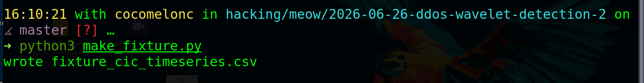
it writes:

fixture_cic_timeseries.csv

C detector

The C program reads:

t,value,label

then it computes:

1. rolling average;
2. Daubechies D4 detail coefficient;
3. robust z-score;
4. event-level metrics.

The most important part is the D4 filter:

static void compute_db4_detail(sample_t *s, int n) {
  const double sqrt3 = 1.7320508075688772935;
  const double denom = 4.0 * 1.4142135623730950488;

  const double h0 = (1.0 + sqrt3) / denom;
  const double h1 = (3.0 + sqrt3) / denom;
  const double h2 = (3.0 - sqrt3) / denom;
  const double h3 = (1.0 - sqrt3) / denom;

  const double g0 = h3;
  const double g1 = -h2;
  const double g2 = h1;
  const double g3 = -h0;

  for (int i = 3; i < n; i++) {
    s[i].db4_detail =
      g0 * s[i - 3].value +
      g1 * s[i - 2].value +
      g2 * s[i - 1].value +
      g3 * s[i].value;
    s[i].db4_detail = fabs(s[i].db4_detail);
  }
}

This is the core idea. Four samples go in, one detail value comes out.

The detector then calibrates a baseline from benign samples before the first attack:

double med = median(baseline, baseline_n);
double sigma = 1.4826 * mad(baseline, baseline_n, med);

then:

samples[i].db4_score = (samples[i].db4_detail - med) / sigma;
samples[i].db4_alert = samples[i].db4_score > db4_threshold;

So, the full source code look like this (hack.c):

demo

Let’s see this in action. First of all, compile:

gcc -O2 -Wall -Wextra hack.c -lm -o hack

run on the local fixture:

./hack fixture_cic_timeseries.csv db4_results.csv 600 8

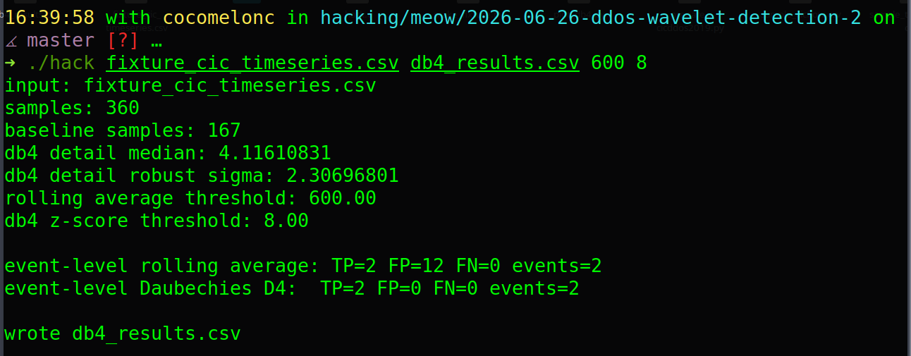
as you can see, in my case:

input: fixture_cic_timeseries.csv
samples: 360
baseline samples: 167
db4 detail median: 4.11610831
db4 detail robust sigma: 2.30696801
rolling average threshold: 600.00
db4 z-score threshold: 8.00

event-level rolling average: TP=2 FP=12 FN=0 events=2
event-level Daubechies D4:  TP=2 FP=0 FN=0 events=2

wrote db4_results.csv

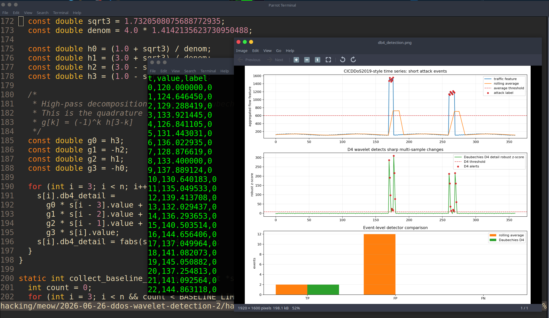
Both methods detected the two attack events. But rolling average produced 12 false post-event alerts because it stays high after the event. D4 produced 0 false events in this test.

this is the main practical result:

rolling average: TP=2 FP=12 FN=0
Daubechies D4:   TP=2 FP=0  FN=0

plot

Generate the plot:

python3 plot_db4.py

result:

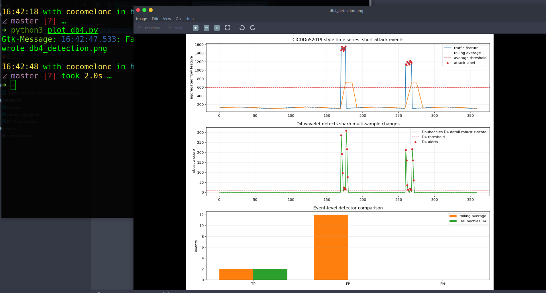
the first plot shows the traffic feature and rolling average. The orange rolling average remains high after the attack ends, which explains the false alert tail.

the second plot shows the Daubechies D4 robust z-score. D4 reacts around the sharp transitions and then returns to baseline quickly.

the third plot compares event-level TP, FP, and FN.

proof that this works

Most of my readers may ask, why this concept works? there are two proofs here: mathematical and experimental.

mathematical proof: rolling average is a smoothing filter. For a short pulse of amplitude \(A \) and duty cycle \(p \):

\[\bar{x}=pA\]

If:

\[pA\le\theta\]

the detector misses or delays the alert.

D4 detail is a high-pass wavelet coefficient:

\[d_t = g_0x_{t-3}+g_1x_{t-2}+g_2x_{t-1}+g_3x_t\]

It suppresses smooth behavior because:

\[\sum g_k=0\]

and:

\[\sum k g_k=0\]

but it reacts to abrupt attack transitions because step-like traffic changes create non-zero high-pass response.

What about experimental proof?

On the local CICDDoS-style test:

rolling average: TP=2 FP=12 FN=0
Daubechies D4:   TP=2 FP=0  FN=0

so in this case D4 preserves detection while reducing false positives:

\[\Delta FP=FP_{avg}-FP_{D4}=12-0=12\]

this is better because an Anti-DDoS detector is not only about finding attacks. It must also avoid unnecessary mitigation after the attack ends.

practical example 2: using real CICDDoS2019 CSV

Now let’s use real data. Download CICDDoS2019 CSV files from the official page:

https://www.unb.ca/cic/datasets/ddos-2019.html

I downloaded part of CICDDoS2019 into:

curl 'https://cicresearch.ca//CICDataset/CICDDoS2019/download.php?file=CSVs%2FCSV-03-11.zip' \
  -H 'User-Agent: Mozilla/5.0 (X11; Linux x86_64; rv:140.0) Gecko/20100101 Firefox/140.0' \
  -H 'Accept: text/html,application/xhtml+xml,application/xml;q=0.9,*/*;q=0.8' \
  -H 'Accept-Language: en-US,en;q=0.5' \
  -H 'Accept-Encoding: gzip, deflate, br, zstd' \
  -H 'Referer: https://cicresearch.ca//CICDataset/CICDDoS2019/browse.php?p=CSVs' \
  -H 'DNT: 1' \
  -H 'Sec-GPC: 1' \
  -H 'Connection: keep-alive' \
  -H 'Cookie: Token=77m9ojfb0piir76m5jtropb6mp' \
  -H 'Upgrade-Insecure-Requests: 1' \
  -H 'Sec-Fetch-Dest: document' \
  -H 'Sec-Fetch-Mode: navigate' \
  -H 'Sec-Fetch-Site: same-origin' \
  -H 'Sec-Fetch-User: ?1' \
  -H 'Priority: u=0, i' --output CICDoS2019-1.zip

curl 'https://cicresearch.ca//CICDataset/CICDDoS2019/download.php?file=CSVs%2FCSV-01-12.zip' \
  -H 'User-Agent: Mozilla/5.0 (X11; Linux x86_64; rv:140.0) Gecko/20100101 Firefox/140.0' \
  -H 'Accept: text/html,application/xhtml+xml,application/xml;q=0.9,*/*;q=0.8' \ 
  -H 'Accept-Language: en-US,en;q=0.5' \
  -H 'Accept-Encoding: gzip, deflate, br, zstd' \
  -H 'Referer: https://cicresearch.ca//CICDataset/CICDDoS2019/browse.php?p=CSVs' \
  -H 'DNT: 1' \
  -H 'Sec-GPC: 1' \
  -H 'Connection: keep-alive' \
  -H 'Cookie: Token=77m9ojfb0piir76m5jtropb6mp' \
  -H 'Upgrade-Insecure-Requests: 1' \
  -H 'Sec-Fetch-Dest: document' \
  -H 'Sec-Fetch-Mode: navigate' \
  -H 'Sec-Fetch-Site: same-origin' \
  -H 'Sec-Fetch-User: ?1' \
  -H 'Priority: u=0, i' --output CICDDoS2019-2.zip

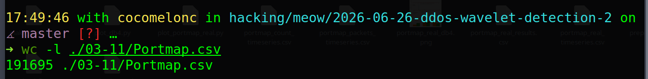
tree ./03-11/

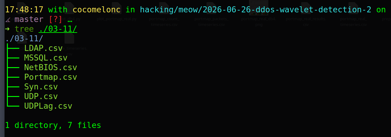
For the first real-data experiment I use Portmap.csv. The reason is pragmatic: it is the smallest file in this folder, but it is still a real CICDDoS2019 CICFlowMeter CSV with Timestamp, more than 80 flow features, and Label.

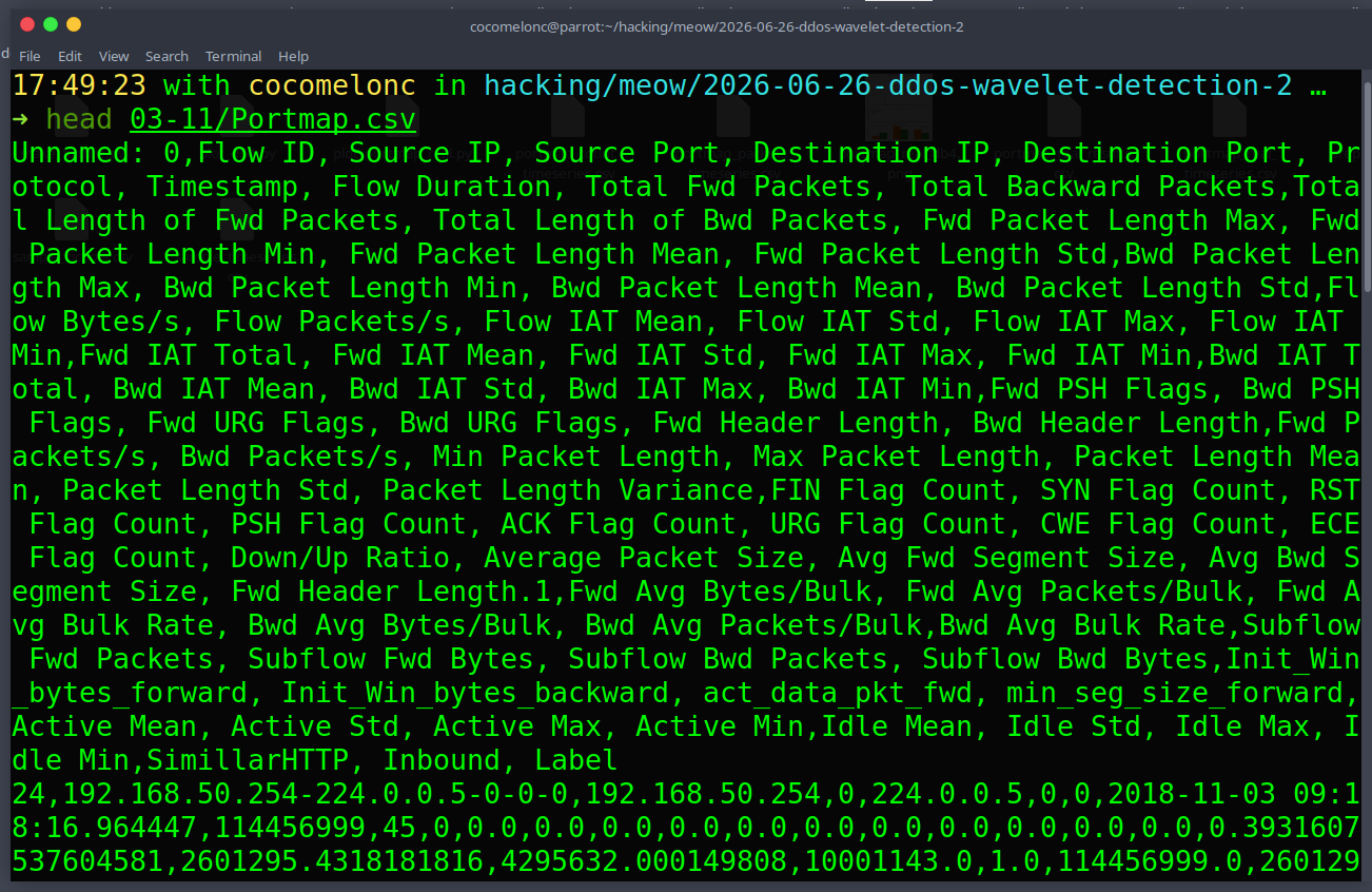
The raw labels include:

BENIGN
Portmap

the input is still too detailed for our wavelet detector because every row is a flow. So the first step is aggregation:

\[x_t = \#\{\text{flows in second }t\}\]

and:

\[y_t = \begin{cases} 1, & \text{at least one Portmap flow exists in second }t \\ 0, & \text{otherwise} \end{cases}\]

I created a dedicated script for this real-data case:

python3 prepare_03_11_real.py --input 03-11/Portmap.csv -o portmap_real_timeseries.csv --attack-label Portmap --feature count

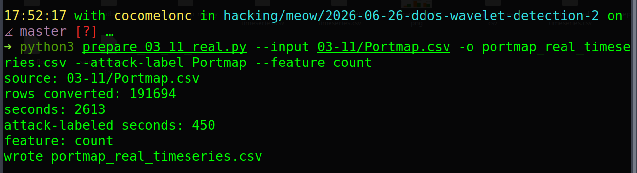
As you can see, on my data:

source: 03-11/Portmap.csv
rows converted: 191694
seconds: 2613
attack-labeled seconds: 450
feature: count
wrote portmap_real_timeseries.csv

The important difference from the synthetic example is baseline calibration. In this real file the first attack label appears almost immediately. So it is wrong to train only on samples before the first attack.

Instead, the new detector learns baseline statistics from all seconds with label=0:

\[B_{avg} = \{\bar{x}_t : y_t=0\}\] \[B_{D4} = \{|d_t| : y_t=0\}\]

Then both detectors use the same robust z-score idea:

\[z^{avg}_t = \frac{\bar{x}_t-\operatorname{median}(B_{avg})} {1.4826\cdot\operatorname{MAD}(B_{avg})}\] \[z^{D4}_t = \frac{|d_t|-\operatorname{median}(B_{D4})} {1.4826\cdot\operatorname{MAD}(B_{D4})}\]

So the comparison is fair: rolling average and D4 both get robust normalization from BENIGN-labeled baseline seconds.

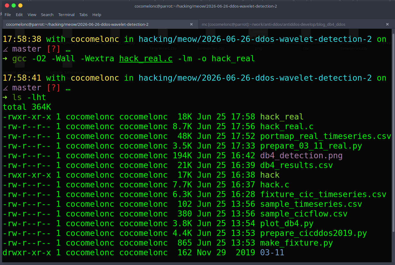
Full source code for real-CSV detector (hack_real.c):

/*
 * hack_real.c
 * Daubechies D4 wavelet detector for real CICDDoS2019-derived time series
 * author @cocomelonc
 *
 * label=0 is BENIGN, label=1 is attack.
 *
 * difference from the toy PoC:
 * - baseline is learned from all BENIGN-labeled seconds, not only from the
 *   prefix before the first attack. This is important for CICDDoS2019 files
 *   where attack traffic may begin very early.
 * - rolling average and DB4 detail are both converted to robust z-scores, so
 *   thresholds are comparable.
 */
#include <ctype.h>
#include <errno.h>
#include <math.h>
#include <stdio.h>
#include <stdlib.h>
#include <string.h>

#define MAX_SAMPLES 400000
#define LINE_MAX_LEN 4096
#define AVG_WINDOW 16
#define EVENT_MERGE_GAP 5
#define EVENT_GRACE 3

typedef struct {
  int t;
  double value;
  int label;
  double rolling_avg;
  double avg_score;
  double db4_detail;
  double db4_score;
  int avg_alert;
  int db4_alert;
} sample_t;

typedef struct {
  int tp;
  int fp;
  int fn;
  int events;
} metrics_t;

static int cmp_double(const void *a, const void *b) {
  double x = *(const double *)a;
  double y = *(const double *)b;
  return (x > y) - (x < y);
}

static double median(double *v, int n) {
  double *tmp = (double *)malloc(sizeof(double) * n);
  if (!tmp) {
    perror("malloc");
    exit(1);
  }
  memcpy(tmp, v, sizeof(double) * n);
  qsort(tmp, n, sizeof(double), cmp_double);

  double result = (n % 2 == 0) ? (tmp[n / 2 - 1] + tmp[n / 2]) / 2.0 : tmp[n / 2];
  free(tmp);
  return result;
}

static double mad(double *v, int n, double med) {
  double *dev = (double *)malloc(sizeof(double) * n);
  if (!dev) {
    perror("malloc");
    exit(1);
  }

  for (int i = 0; i < n; i++) {
    dev[i] = fabs(v[i] - med);
  }

  double result = median(dev, n);
  free(dev);
  return result < 1e-9 ? 1e-9 : result;
}

static char *trim(char *s) {
  while (isspace((unsigned char)*s)) {
    s++;
  }
  if (*s == 0) {
    return s;
  }

  char *end = s + strlen(s) - 1;
  while (end > s && isspace((unsigned char)*end)) {
    *end = 0;
    end--;
  }
  return s;
}

static int read_series(const char *path, sample_t *samples) {
  FILE *f = fopen(path, "r");
  if (!f) {
    fprintf(stderr, "failed to open %s: %s\n", path, strerror(errno));
    exit(1);
  }

  char line[LINE_MAX_LEN];
  int n = 0;
  int line_no = 0;

  while (fgets(line, sizeof(line), f)) {
    line_no++;
    char *p = trim(line);
    if (*p == 0) {
      continue;
    }
    if (line_no == 1 && strstr(p, "t") && strstr(p, "value")) {
      continue;
    }

    char *t_s = strtok(p, ",");
    char *value_s = strtok(NULL, ",");
    char *label_s = strtok(NULL, ",");
    if (!t_s || !value_s || !label_s) {
      fprintf(stderr, "invalid CSV line %d\n", line_no);
      exit(1);
    }
    if (n >= MAX_SAMPLES) {
      fprintf(stderr, "too many samples, max=%d\n", MAX_SAMPLES);
      exit(1);
    }

    samples[n].t = atoi(trim(t_s));
    samples[n].value = atof(trim(value_s));
    samples[n].label = atoi(trim(label_s)) != 0;
    n++;
  }

  fclose(f);
  return n;
}

static void compute_rolling_avg(sample_t *s, int n) {
  for (int i = 0; i < n; i++) {
    int start = i - AVG_WINDOW + 1;
    if (start < 0) {
      start = 0;
    }

    double sum = 0.0;
    int count = 0;
    for (int j = start; j <= i; j++) {
      sum += s[j].value;
      count++;
    }
    s[i].rolling_avg = sum / (double)count;
  }
}

static void compute_db4_detail(sample_t *s, int n) {
  const double sqrt3 = 1.7320508075688772935;
  const double denom = 4.0 * 1.4142135623730950488;

  const double h0 = (1.0 + sqrt3) / denom;
  const double h1 = (3.0 + sqrt3) / denom;
  const double h2 = (3.0 - sqrt3) / denom;
  const double h3 = (1.0 - sqrt3) / denom;

  const double g0 = h3;
  const double g1 = -h2;
  const double g2 = h1;
  const double g3 = -h0;

  for (int i = 3; i < n; i++) {
    s[i].db4_detail =
      g0 * s[i - 3].value +
      g1 * s[i - 2].value +
      g2 * s[i - 1].value +
      g3 * s[i].value;
    s[i].db4_detail = fabs(s[i].db4_detail);
  }
}

static int collect_benign_feature(sample_t *s, int n, double *out, int feature) {
  int count = 0;
  for (int i = 0; i < n; i++) {
    if (s[i].label) {
      continue;
    }
    out[count++] = (feature == 0) ? s[i].rolling_avg : s[i].db4_detail;
  }
  return count;
}

static metrics_t event_metrics(sample_t *s, int n, int use_db4) {
  metrics_t m = {0, 0, 0, 0};
  unsigned char *covered = (unsigned char *)calloc(n, sizeof(unsigned char));
  if (!covered) {
    perror("calloc");
    exit(1);
  }

  int i = 0;
  while (i < n) {
    if (!s[i].label) {
      i++;
      continue;
    }

    int start = i;
    int end = i;
    int last_attack = i;
    i++;

    while (i < n) {
      if (s[i].label) {
        last_attack = i;
        end = i;
        i++;
        continue;
      }
      if (i - last_attack <= EVENT_MERGE_GAP) {
        end = i;
        i++;
        continue;
      }
      break;
    }

    int grace_end = end + EVENT_GRACE;
    if (grace_end >= n) {
      grace_end = n - 1;
    }

    int detected = 0;
    for (int j = start; j <= grace_end; j++) {
      covered[j] = 1;
      int alert = use_db4 ? s[j].db4_alert : s[j].avg_alert;
      if (alert) {
        detected = 1;
      }
    }

    m.events++;
    if (detected) {
      m.tp++;
    } else {
      m.fn++;
    }
  }

  for (i = 0; i < n; i++) {
    int alert = use_db4 ? s[i].db4_alert : s[i].avg_alert;
    if (alert && !covered[i]) {
      m.fp++;
    }
  }

  free(covered);
  return m;
}

static void write_results(const char *path, sample_t *s, int n) {
  FILE *f = fopen(path, "w");
  if (!f) {
    fprintf(stderr, "failed to open %s: %s\n", path, strerror(errno));
    exit(1);
  }

  fprintf(f, "t,value,label,rolling_avg,avg_score,db4_detail,db4_score,avg_alert,db4_alert\n");
  for (int i = 0; i < n; i++) {
    fprintf(f, "%d,%.8f,%d,%.8f,%.8f,%.8f,%.8f,%d,%d\n",
      s[i].t,
      s[i].value,
      s[i].label,
      s[i].rolling_avg,
      s[i].avg_score,
      s[i].db4_detail,
      s[i].db4_score,
      s[i].avg_alert,
      s[i].db4_alert);
  }
  fclose(f);
}

int main(int argc, char **argv) {
  const char *input = "portmap_count_timeseries.csv";
  const char *output = "portmap_real_results.csv";
  double avg_threshold = 8.0;
  double db4_threshold = 8.0;

  if (argc > 1) {
    input = argv[1];
  }
  if (argc > 2) {
    output = argv[2];
  }
  if (argc > 3) {
    avg_threshold = atof(argv[3]);
  }
  if (argc > 4) {
    db4_threshold = atof(argv[4]);
  }

  sample_t *samples = (sample_t *)calloc(MAX_SAMPLES, sizeof(sample_t));
  if (!samples) {
    perror("calloc");
    return 1;
  }

  int n = read_series(input, samples);
  if (n < 32) {
    fprintf(stderr, "need at least 32 samples\n");
    free(samples);
    return 1;
  }

  compute_rolling_avg(samples, n);
  compute_db4_detail(samples, n);

  double *benign_avg = (double *)malloc(sizeof(double) * n);
  double *benign_db4 = (double *)malloc(sizeof(double) * n);
  if (!benign_avg || !benign_db4) {
    perror("malloc");
    free(samples);
    return 1;
  }

  int benign_avg_n = collect_benign_feature(samples, n, benign_avg, 0);
  int benign_db4_n = collect_benign_feature(samples, n, benign_db4, 1);
  if (benign_avg_n < 16 || benign_db4_n < 16) {
    fprintf(stderr, "not enough benign samples\n");
    free(benign_avg);
    free(benign_db4);
    free(samples);
    return 1;
  }

  double avg_med = median(benign_avg, benign_avg_n);
  double avg_sigma = 1.4826 * mad(benign_avg, benign_avg_n, avg_med);
  double db4_med = median(benign_db4, benign_db4_n);
  double db4_sigma = 1.4826 * mad(benign_db4, benign_db4_n, db4_med);

  for (int i = 0; i < n; i++) {
    samples[i].avg_score = (samples[i].rolling_avg - avg_med) / avg_sigma;
    samples[i].db4_score = (samples[i].db4_detail - db4_med) / db4_sigma;
    samples[i].avg_alert = samples[i].avg_score > avg_threshold;
    samples[i].db4_alert = samples[i].db4_score > db4_threshold;
  }

  metrics_t avg_m = event_metrics(samples, n, 0);
  metrics_t db4_m = event_metrics(samples, n, 1);

  printf("input: %s\n", input);
  printf("samples: %d\n", n);
  printf("benign samples for baseline: %d\n", benign_avg_n);
  printf("rolling avg median: %.8f robust sigma: %.8f threshold z: %.2f\n",
    avg_med, avg_sigma, avg_threshold);
  printf("db4 detail median: %.8f robust sigma: %.8f threshold z: %.2f\n\n",
    db4_med, db4_sigma, db4_threshold);

  printf("event-level rolling average z-score: TP=%d FP=%d FN=%d events=%d\n",
    avg_m.tp, avg_m.fp, avg_m.fn, avg_m.events);
  printf("event-level Daubechies D4 z-score:  TP=%d FP=%d FN=%d events=%d\n",
    db4_m.tp, db4_m.fp, db4_m.fn, db4_m.events);

  write_results(output, samples, n);
  printf("\nwrote %s\n", output);

  free(benign_avg);
  free(benign_db4);
  free(samples);
  return 0;
}

demo 2

Let’s see this in action, compile the real-data detector:

gcc -O2 -Wall -Wextra hac_real.c -lm -o hack_real

Then, run with the same z-threshold for both detectors:

./hack_real portmap_real_timeseries.csv portmap_real_results.csv 4 4

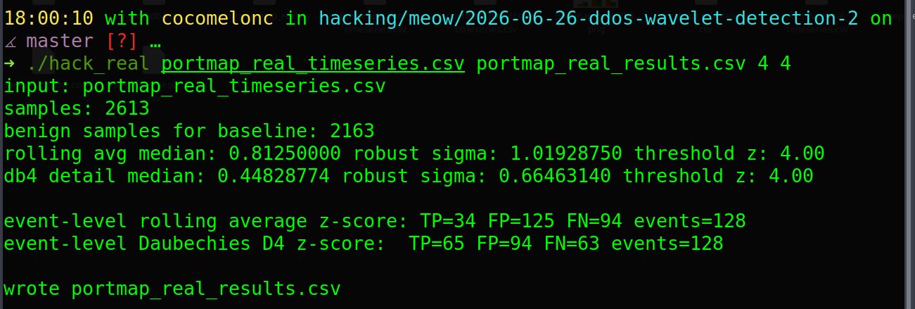
As you can see, in my case:

input: portmap_real_timeseries.csv
samples: 2613
benign samples for baseline: 2163
rolling avg median: 0.81250000 robust sigma: 1.01928750 threshold z: 4.00
db4 detail median: 0.44828774 robust sigma: 0.66463140 threshold z: 4.00

event-level rolling average z-score: TP=34 FP=125 FN=94 events=128
event-level Daubechies D4 z-score:  TP=65 FP=94 FN=63 events=128

wrote portmap_real_results.csv

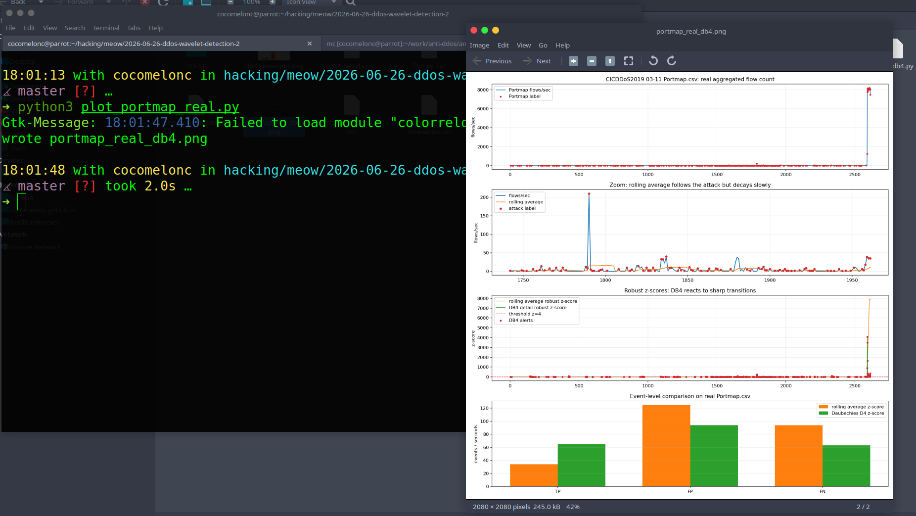
Finally, draw the real-data plot:

python3 plot_portmap_real.py

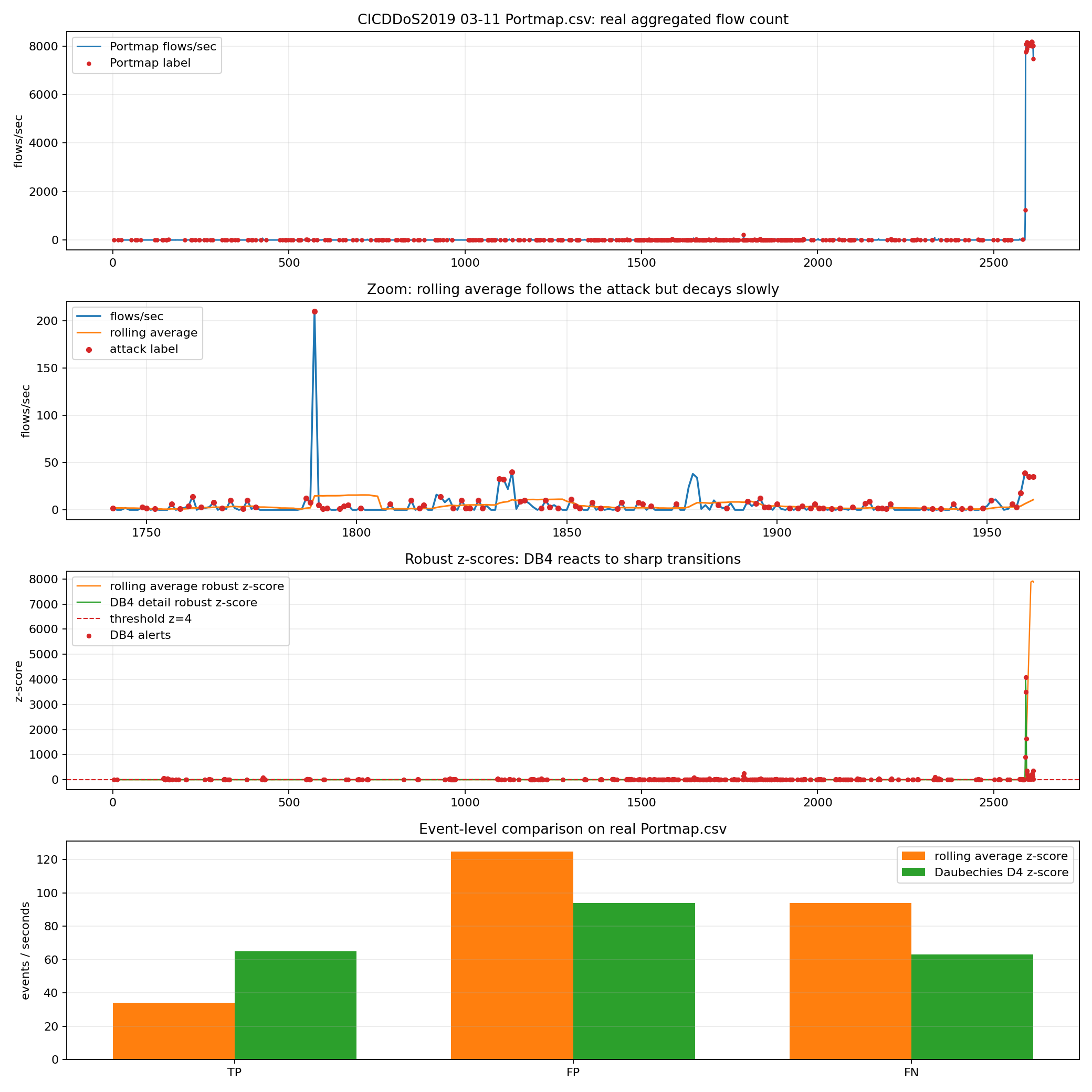
The first plot is the real aggregated flow count from 03-11/Portmap.csv.

The second plot zooms into an attack-heavy area. You can see short labeled attack points mixed with small baseline traffic. This is much messier than the synthetic example, as expected from a real dataset.

The third plot compares robust z-scores:

orange: rolling average z-score;
green: Daubechies D4 detail z-score;
dashed red line: threshold \( z=4 \).

The last plot shows event-level metrics.

proof that this works (example 2)

If you’ve made it this far, let’s prove again why it works here.

Mathematical proof:

Rolling average is a smoothing filter:

\[\bar{x}_t=\frac{1}{W}\sum_{i=0}^{W-1}x_{t-i}\]

this is useful for long high-volume attacks, but it has inertia. If traffic jumps and then quickly returns to normal, the average can remain elevated because old attack samples still live inside the window.

D4 detail is a high-pass wavelet coefficient:

\[d_t = g_0x_{t-3}+g_1x_{t-2}+g_2x_{t-1}+g_3x_t\]

It suppresses smooth behavior because:

\[\sum_{k=0}^{3}g_k=0\]

and:

\[\sum_{k=0}^{3}k g_k=0\]

So for a constant or nearly linear local trend, D4 detail is small. But for an abrupt traffic transition, D4 detail becomes large. In cybersecurity language:

rolling average asks: is traffic high for a while?
D4 asks: did the traffic shape suddenly break?

practical proof on the real 03-11/Portmap.csv:

rolling average z-score: TP=34 FP=125 FN=94
Daubechies D4 z-score:  TP=65 FP=94  FN=63

At the same threshold \( z=4 \), D4 is better on all three event-level metrics:

\[TP_{D4}-TP_{avg}=65-34=31\] \[FP_{avg}-FP_{D4}=125-94=31\] \[FN_{avg}-FN_{D4}=94-63=31\]

So on this real file from dataset, D4 finds more Portmap attack events and produces fewer false positives and fewer misses.

This does not mean D4 is universally better for every DDoS type. It means something narrower and defensible:

For this CICDDoS2019 Portmap.csv flow-count time series, with BENIGN-based robust normalization and equal threshold (z=4), Daubechies D4 dominates rolling average in event-level TP/FP/FN.

That is the kind of claim we can publish honestly.

The detection success depends on:

• the selected traffic feature, here flows/sec;
• the quality of labels;
• the event merge window, here 5 seconds;
• the grace window after an event, here 3 seconds;
• the z-threshold, here 4;
• whether the attack creates abrupt transitions or only a very slow ramp.

for a full paper-style evaluation, repeat the same experiment for:

• Syn.csv;
• UDP.csv;
• UDPLag.csv;
• LDAP.csv;
• MSSQL.csv;
• NetBIOS.csv.

Then plot ROC/PR curves across multiple thresholds:

\[TPR(\tau)=\frac{TP(\tau)}{TP(\tau)+FN(\tau)}\] \[FPR(\tau)=\frac{FP(\tau)}{FP(\tau)+TN(\tau)}\] \[\operatorname{Precision}(\tau)=\frac{TP(\tau)}{TP(\tau)+FP(\tau)}\]

This is how to prove whether the method generalizes beyond one file.

limitations

this detector is not a complete Anti-DDoS system.

D4 wavelet is good for abrupt changes. It is not enough for:

• very slow ramp attacks;
• application-layer attacks with low traffic volume;
• attacks where the signal is not rate but distribution;
• attacks hidden inside normal event traffic.

For those, we need more features:

\[S = w_1Z_{rate}+ w_2Z_{D4}+ w_3Z_{entropy}+ w_4Z_{protocol}\]

For example:

• SYN flood: handshake asymmetry;
• DNS flood: qname entropy and NXDOMAIN ratio;
• UDP reflection: packet size and source port distribution;
• carpet bombing: destination distribution and matrix anomalies.

conclusion

Haar wavelet is good for explaining the idea. Daubechies D4 is a better next step because it is still simple but has stronger mathematical properties.

In this post:

• we implemented D4 in C;
• we used robust median/MAD thresholding;
• we prepared a CICDDoS2019-compatible time-series format;
• we added a converter for real CICDDoS2019 flow CSV;
• we plotted traffic, D4 score, and event-level metrics;
• we showed that D4 can reduce false post-event alerts compared with rolling average.

This is a useful building block for a defensive Anti-DDoS research pipeline.

references and further reading

If you want to go deeper into the math and the research behind this post, here are the academic papers I recommend. I grouped them by topic.

Wavelets and signal analysis of network traffic

P. Barford, J. Kline, D. Plonka, A. Ron. A Signal Analysis of Network Traffic Anomalies (ACM SIGCOMM Internet Measurement Workshop, 2002) - pdf. The classic paper on using wavelet decomposition to expose short-lived traffic anomalies.
S. Mallat. A Theory for Multiresolution Signal Decomposition: The Wavelet Representation (IEEE Trans. PAMI, 1989) - doi. The foundational multiresolution analysis paper behind the Haar/DWT machinery.
I. Daubechies. Ten Lectures on Wavelets (SIAM, 1992) - doi. The standard reference textbook for wavelet theory.
C.-M. Cheng, H. T. Kung, K.-S. Tan. Use of Spectral Analysis in Defense Against DoS Attacks (IEEE GLOBECOM, 2002) - pdf. Spectral/power-density view of DoS traffic, a close cousin of the wavelet approach.

Low-rate and pulsing DDoS attacks

A. Kuzmanovic, E. W. Knightly. Low-Rate TCP-Targeted Denial of Service Attacks (The Shrew vs. the Mice and Elephants) (ACM SIGCOMM, 2003) - pdf. Explains exactly why low duty-cycle pulses evade average-based detectors while still hurting TCP.

Change-point detection (onset detection)

E. S. Page. Continuous Inspection Schemes (Biometrika, 1954) - doi. The original CUSUM change-detection scheme.
G. V. Moustakides. Optimal Stopping Times for Detecting Changes in Distributions (Annals of Statistics, 1986) - doi. Proves the minimax optimality of CUSUM for minimum-delay detection.
H. Wang, D. Zhang, K. G. Shin. Detecting SYN Flooding Attacks (IEEE INFOCOM, 2002) - pdf. Non-parametric CUSUM applied to the SYN-FIN difference; directly relevant to SYN-flood detection.

Entropy and statistical / distributional detection

L. Feinstein, D. Schnackenberg, R. Balupari, D. Kindred. Statistical Approaches to DDoS Attack Detection and Response (DARPA DISCEX, 2003) - doi. Entropy and chi-square tests for volume-independent detection.
A. Lall, V. Sekar, M. Ogihara, J. Xu, H. Zhang. Data Streaming Algorithms for Estimating Entropy of Network Traffic (ACM SIGMETRICS, 2006) - pdf. How to estimate traffic entropy at line rate with small memory.
A. Lakhina, M. Crovella, C. Diot. Diagnosing Network-Wide Traffic Anomalies (ACM SIGCOMM, 2004) - pdf. PCA subspace method for correlated, network-wide anomalies.

Robust statistics (median / MAD / z-score)

P. J. Huber. Robust Estimation of a Location Parameter (Annals of Mathematical Statistics, 1964) - doi. The origin of robust location estimation behind median/MAD.
F. R. Hampel. The Influence Curve and Its Role in Robust Estimation (JASA, 1974) - doi. Breakdown point and influence functions, why MAD beats standard deviation under contamination.

Baseline modeling and seasonality

J. D. Brutlag. Aberrant Behavior Detection in Time Series for Network Monitoring (USENIX LISA, 2000) - pdf. Holt-Winters seasonal baselining with confidence bands - the operational version of an adaptive threshold.

Self-similar traffic (background for why wavelets fit network data)

W. E. Leland, M. S. Taqqu, W. Willinger, D. V. Wilson. On the Self-Similar Nature of Ethernet Traffic (ACM SIGCOMM, 1993) - doi. Shows network traffic is self-similar/bursty across scales, which motivates multi-resolution analysis.

Surveys and datasets

J. Mirkovic, P. Reiher. A Taxonomy of DDoS Attack and DDoS Defense Mechanisms (ACM SIGCOMM CCR, 2004) - doi. A good map of the whole attack/defense landscape.
I. Sharafaldin, A. H. Lashkari, S. Hakak, A. A. Ghorbani. Developing Realistic Distributed Denial of Service (DDoS) Attack Dataset and Taxonomy (IEEE ICCST, 2019) - doi. The paper behind the CICDDoS2019 dataset linked above.

Haar wavelet
Daubechies wavelet
Wavelet
source code in github

This is a practical defensive case for educational purposes only.

Thanks for your time happy hacking and good bye!
PS. All drawings and screenshots are mine