Malware shellcode delivery via signal - part 5. Physics-guided AI demodulator. PyTorch example
﷽
Hello, cybersecurity enthusiasts and white hackers!
In part 4, I embedded a Bell 202 FSK frame into music, encoded it as MP3, and recovered it with a classical Goertzel receiver. The receiver worked, but the experiment also exposed the usual acoustic-channel problems: frequency drift, narrow-band interference, multipath, clipping, impulsive noise, and imperfect symbol boundaries.
Today I want to test a practical question: can a tiny neural network make the FSK decision more robust without throwing away the DSP knowledge we already have?
The short answer from my first NVIDIA L20 experiment is: a neural network can help, but only if we give it the right inductive bias. A raw waveform CNN was worse than Goertzel. A hybrid receiver with a fixed quadrature filter bank and a small learned head reduced the relative bit error rate by about 14% in my synthetic noisy and stress tests.
This is a decode-only laboratory experiment. The example payload is harmless text, recovered bytes are never mapped as executable memory, and the model is evaluated as a demodulator rather than an execution component. An audio file by itself does not execute anything; a separate receiver must already be present.
why add AI to a two-tone modem?
For an aligned Bell 202 symbol, the classical receiver has a wonderfully simple rule. Measure energy at 1200 Hz, measure energy at 2200 Hz, and choose the larger value:
Using quadrature correlation, the energy at frequency \(f\) is:
\[P_f = \left(\sum_{n=0}^{N-1}x[n]\cos(2\pi fn/F_s)\right)^2 + \left(\sum_{n=0}^{N-1}x[n]\sin(2\pi fn/F_s)\right)^2.\]At 48000 Hz and 300 baud, one nominal symbol contains:
In code this whole rule is just two correlations per tone. Here is goertzel_predict from fsk_ai_benchmark.py, the exact baseline used in the benchmark:
@torch.inference_mode()
def goertzel_predict(x):
    # Correlation form of the two-bin Goertzel detector.
    device = x.device
    t = torch.arange(N, device=device).float() / FS
    wave = torch.stack([
        torch.cos(2 * math.pi * F0 * t), torch.sin(2 * math.pi * F0 * t),
        torch.cos(2 * math.pi * F1 * t), torch.sin(2 * math.pi * F1 * t),
    ])
    z = x[:, 0, :] @ wave.T
    p0 = z[:, 0].square() + z[:, 1].square()
    p1 = z[:, 2].square() + z[:, 3].square()
    return (p1 > p0).long()
The two square() sums are exactly \(P_{1200}\) and \(P_{2200}\) from the formula above, and the last line is the decision rule p1 > p0. That is the entire classical receiver.
This detector is fast, explainable, and almost impossible to beat on a clean channel. The interesting case is not the clean channel. Suppose the 1200 Hz tone arrives at 1280 Hz, a short click corrupts one quarter of the symbol, and music creates a stronger peak near one of our decision frequencies. A detector that sees only two scalar powers discards useful context.
The AI idea is therefore not to replace DSP. It is to keep a bank of physically meaningful measurements and learn how to combine them.
the first attempt: raw waveform CNN
My first model received all 160 waveform samples directly:
self.net = nn.Sequential(
    nn.Conv1d(1, 16, 9, stride=2, padding=4),
    nn.BatchNorm1d(16), nn.SiLU(),
    nn.Conv1d(16, 32, 7, stride=2, padding=3),
    nn.BatchNorm1d(32), nn.SiLU(),
    nn.Conv1d(32, 64, 5, stride=2, padding=2),
    nn.BatchNorm1d(64), nn.SiLU(),
    nn.AdaptiveAvgPool1d(1),
    nn.Flatten(),
    nn.Linear(64, 2),
)
It had only 14,434 trainable parameters and trained in 12.19 seconds on the L20. It also failed to beat the simple baseline:
| test channel | nominal Goertzel BER | raw CNN BER |
|---|---|---|
| clean | 0.0000% |
0.0000% |
| noisy | 4.4340% |
7.6645% |
| stress | 17.1810% |
22.3980% |
These values came from the preliminary run and its own random test draw, so they should not be mixed directly with the final table below. The conclusion is still clear: a generic CNN did not discover a better receiver merely because I gave it millions of synthetic symbols.
This negative result changed the architecture. Instead of asking the model to rediscover Fourier analysis from scratch, I made the DSP front end explicit.
synthetic acoustic channel
For the initial benchmark I generated labeled FSK symbols directly on the GPU. Each clean symbol begins as:
\[s_b[n] = A\sin\left(2\pi(f_b + \Delta f)n/F_s + \phi\right),\]where \(f_b\) is 1200 or 2200 Hz, \(\Delta f\) is frequency offset, \(A\) is random gain, and \(\phi\) is random phase. The channel then adds a delayed copy, an interfering tone, Gaussian noise, occasional impulsive corruption, DC offset, and soft clipping:
The three evaluation modes are:
| mode | purpose |
|---|---|
clean |
controlled sanity check with only light noise |
noisy |
the same impairment ranges used for training |
stress |
harder frequency offset, noise, echo, interference, and clicks |
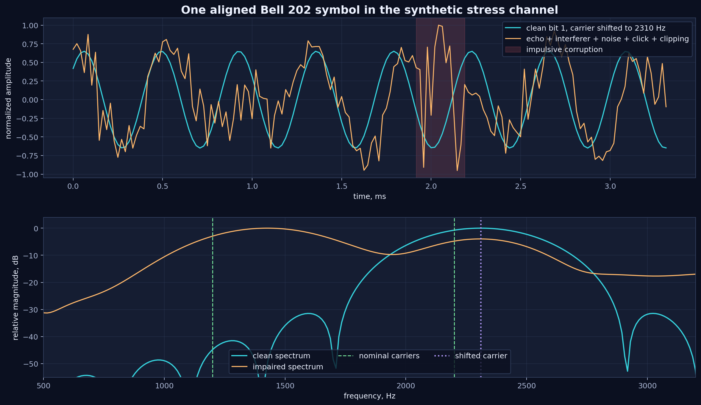
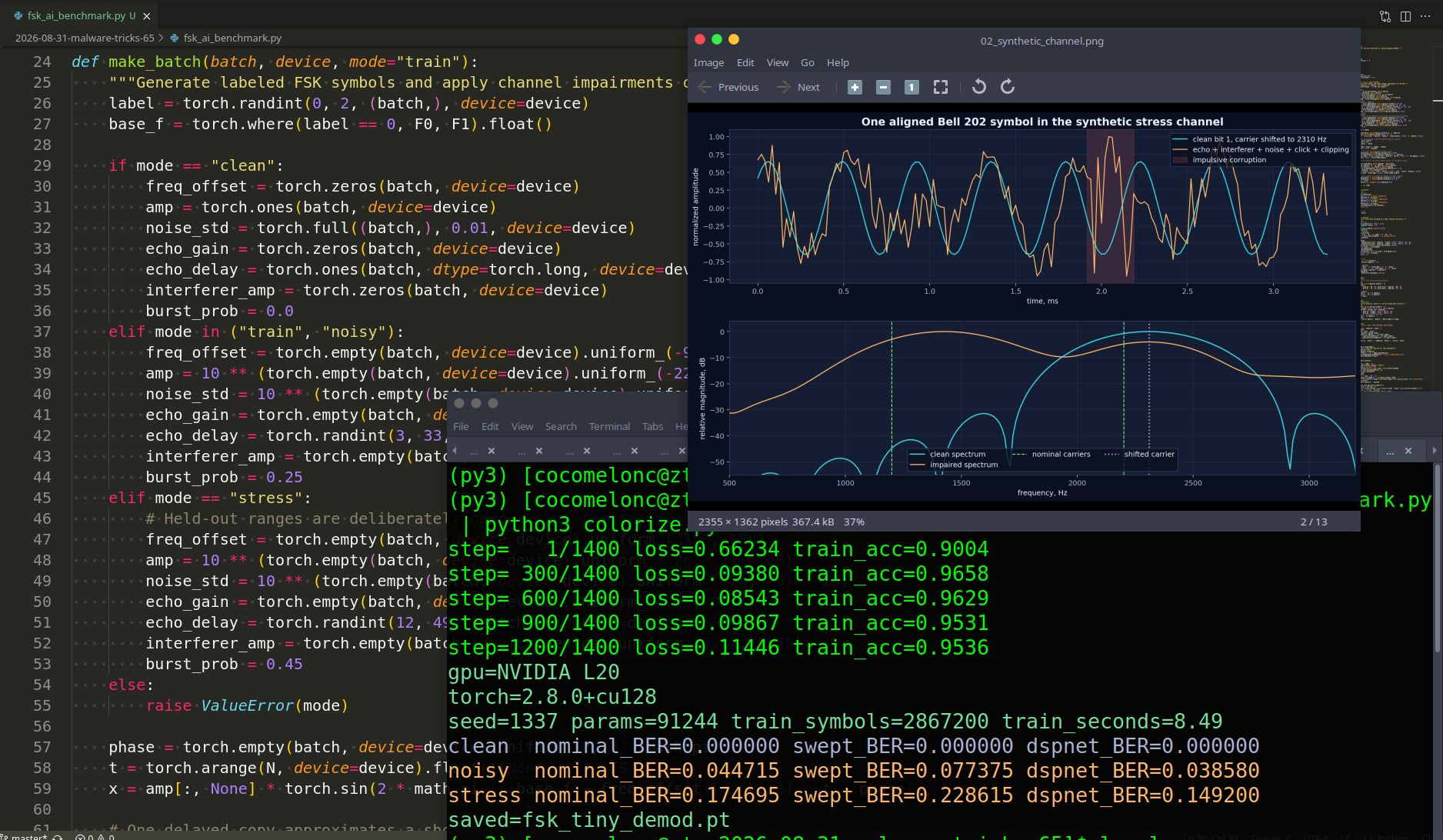
The training distribution used frequency offsets up to ±90 Hz, gain from -22 to 0 dB, echo gain up to 0.55, random narrow-band interference, and impulsive corruption in 25% of the symbols. The stress set extended several of those ranges, including offsets up to ±150 Hz and echo gain up to 0.75.
The important point is that no malware samples are needed for training. Bits are bits. The model learns the channel and the modulation, not payload semantics.
The whole benchmark lives in one file, fsk_ai_benchmark.py. It opens by pinning the sample rate, the symbol length, the two Bell 202 tones, and the random seed, so every run is reproducible:
import math
import random
import time

import torch
import torch.nn as nn
import torch.nn.functional as F

SEED = 1337
FS = 48_000       # sample rate, Hz
N = 160           # samples per symbol (48000 / 300 baud)
F0 = 1_200.0      # bit 0 tone (Bell 202 mark), Hz
F1 = 2_200.0      # bit 1 tone (Bell 202 space), Hz

random.seed(SEED)
torch.manual_seed(SEED)
torch.cuda.manual_seed_all(SEED)
torch.backends.cudnn.benchmark = True
The make_batch helper turns those constants into labeled symbols and applies the channel model from the two equations above. The clean tone becomes x, every impairment is added on top of it, and the final torch.tanh is exactly the soft clipping \(g(\cdot)\) in \(y[n]\):
def make_batch(batch, device, mode="train"):
    """Generate labeled FSK symbols and apply channel impairments on the GPU."""
    label = torch.randint(0, 2, (batch,), device=device)
    base_f = torch.where(label == 0, F0, F1).float()

    if mode == "clean":
        freq_offset = torch.zeros(batch, device=device)
        amp = torch.ones(batch, device=device)
        noise_std = torch.full((batch,), 0.01, device=device)
        echo_gain = torch.zeros(batch, device=device)
        echo_delay = torch.ones(batch, dtype=torch.long, device=device)
        interferer_amp = torch.zeros(batch, device=device)
        burst_prob = 0.0
    elif mode in ("train", "noisy"):
        freq_offset = torch.empty(batch, device=device).uniform_(-90, 90)
        amp = 10 ** (torch.empty(batch, device=device).uniform_(-22, 0) / 20)
        noise_std = 10 ** (torch.empty(batch, device=device).uniform_(-30, -8) / 20)
        echo_gain = torch.empty(batch, device=device).uniform_(0, 0.55)
        echo_delay = torch.randint(3, 33, (batch,), device=device)
        interferer_amp = torch.empty(batch, device=device).uniform_(0, 0.28)
        burst_prob = 0.25
    elif mode == "stress":
        # Held-out ranges are deliberately harder than the training distribution.
        freq_offset = torch.empty(batch, device=device).uniform_(-150, 150)
        amp = 10 ** (torch.empty(batch, device=device).uniform_(-26, -2) / 20)
        noise_std = 10 ** (torch.empty(batch, device=device).uniform_(-24, -5) / 20)
        echo_gain = torch.empty(batch, device=device).uniform_(0.25, 0.75)
        echo_delay = torch.randint(12, 49, (batch,), device=device)
        interferer_amp = torch.empty(batch, device=device).uniform_(0.12, 0.45)
        burst_prob = 0.45
    else:
        raise ValueError(mode)

    phase = torch.empty(batch, device=device).uniform_(0, 2 * math.pi)
    t = torch.arange(N, device=device).float()[None, :] / FS
    x = amp[:, None] * torch.sin(2 * math.pi * (base_f + freq_offset)[:, None] * t + phase[:, None])

    # One delayed copy approximates a short multipath acoustic channel.
    delayed = torch.zeros_like(x)
    for delay in range(3, 49):
        mask = echo_delay == delay
        if mask.any():
            delayed[mask, delay:] = x[mask, :-delay]
    x = x + echo_gain[:, None] * delayed

    # A narrow-band interferer and broadband Gaussian noise.
    int_f = torch.empty(batch, device=device).uniform_(700, 2_700)
    int_phase = torch.empty(batch, device=device).uniform_(0, 2 * math.pi)
    x = x + interferer_amp[:, None] * torch.sin(2 * math.pi * int_f[:, None] * t + int_phase[:, None])
    x = x + noise_std[:, None] * torch.randn_like(x)

    # Short impulsive corruption: fan click, buffer glitch, or microphone knock.
    if burst_prob:
        active = torch.rand(batch, device=device) < burst_prob
        start = torch.randint(0, N - 20, (batch,), device=device)
        width = torch.randint(4, 21, (batch,), device=device)
        burst_amp = torch.empty(batch, device=device).uniform_(0.2, 1.2)
        idx = torch.arange(N, device=device)[None, :]
        burst_mask = active[:, None] & (idx >= start[:, None]) & (idx < (start + width)[:, None])
        x = x + burst_mask * burst_amp[:, None] * torch.randn_like(x)

    # Random DC and soft clipping are common in inexpensive capture paths.
    x = x + torch.empty(batch, 1, device=device).uniform_(-0.08, 0.08)
    drive = torch.empty(batch, 1, device=device).uniform_(0.8, 2.0)
    x = torch.tanh(x * drive)
    peak = x.abs().amax(dim=1, keepdim=True).clamp_min(1e-5)
    x = x / peak
    return x[:, None, :], label
physics-guided front end
The improved receiver measures quadrature energy on a dense filter bank from 700 Hz to 2700 Hz in 25 Hz steps. It does this once over the complete symbol and once over each of four quarters.
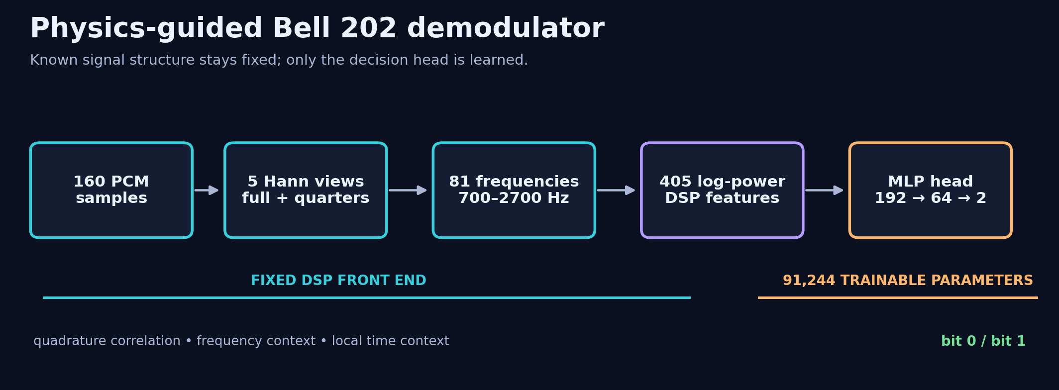
Read the pipeline from left to right. One Bell 202 symbol contributes 160 PCM samples. Five Hann-windowed views of the same symbol - one full-length view and four quarter-symbol views - are correlated with 81 candidate frequencies. This produces 5 × 81 = 405 log-power measurements that preserve both frequency context and coarse time context. Everything up to those 405 features is fixed DSP; training changes only the 91,244 parameters in the MLP decision head. The network therefore never has to rediscover the carrier frequencies or quadrature correlation from raw audio.
For frequency bin \(f_k\) and time mask \(w_m[n]\):
\[E_{m,k} = \log\left(1 + \left(\sum_n w_m[n]x[n]\cos(2\pi f_kn/F_s)\right)^2 + \left(\sum_n w_m[n]x[n]\sin(2\pi f_kn/F_s)\right)^2 \right).\]The full-symbol features show frequency drift. The four shorter views let the model reduce the influence of a click or short dropout. A small MLP then combines the 405 log-power features:
class DSPTinyDemod(nn.Module):
    def __init__(self):
        super().__init__()
        freqs = torch.arange(700.0, 2700.1, 25.0)
        t = torch.arange(160).float() / 48000

        windows = [torch.hann_window(160, periodic=False)]
        for part in range(4):
            w = torch.zeros(160)
            lo, hi = part * 40, (part + 1) * 40
            w[lo:hi] = torch.hann_window(40, periodic=False)
            windows.append(w)

        kernels = []
        for w in windows:
            kernels.append(
                torch.cos(2 * torch.pi * freqs[:, None] * t[None, :]) * w
            )
            kernels.append(
                torch.sin(2 * torch.pi * freqs[:, None] * t[None, :]) * w
            )

        self.register_buffer("kernels", torch.cat(kernels))
        self.head = nn.Sequential(
            nn.LayerNorm(405),
            nn.Linear(405, 192), nn.SiLU(), nn.Dropout(0.05),
            nn.Linear(192, 64), nn.SiLU(),
            nn.Linear(64, 2),
        )

    def forward(self, x):
        z = x[:, 0, :] @ self.kernels.T
        powers = []

        for part in range(5):
            begin = part * 162
            c = z[:, begin:begin + 81]
            s = z[:, begin + 81:begin + 162]
            powers.append(torch.log1p(c.square() + s.square()))

        return self.head(torch.cat(powers, dim=1))
Only 91,244 parameters are trainable. The sinusoidal filter bank is fixed. This makes the model small, inspectable, and much easier to reason about than an end-to-end waveform network.
the math of the learned decision
The DSP front end gives us 405 numbers per symbol. The learned part is small, and its math is simpler than it looks. Let me write it out for readers who are new to machine learning.
The model is just a function. - our receiver is a function \(f_\theta\) that maps one symbol \(x\) (the 160 samples) to a decision. It has two stages:
Here \(\Phi(x)\) is the fixed quadrature filter bank. It turns 160 samples into 405 log-power features and never changes during training. \(\text{head}_\theta\) is the tiny MLP with trainable weights \(\theta\). In one sentence: physics computes the features, and training only learns how to weigh them.
Logits and softmax. - the last layer nn.Linear(64, 2) outputs two raw numbers \(z_0, z_1\), called logits. They are not probabilities yet. We turn them into probabilities with the softmax function:
Now \(p_0 + p_1 = 1\), and the decoded bit is simply the larger one:
\[\hat b = \arg\max_i p_i.\]Cross-entropy loss. - during training we need one number that says how wrong the model is. If the true bit is \(b\), the loss for one symbol is:
\[\mathcal{L} = -\log p_b.\]If the model is confident and correct, \(p_b \approx 1\) and the loss is near 0. If it is confident and wrong, \(p_b \approx 0\) and the loss is large. This is exactly what F.cross_entropy computes in the training loop. Over a batch of \(M\) symbols we take the average:
Learning means minimizing the loss. - training looks for the weights that make the average loss small:
\[\theta^\star = \arg\min_\theta \; \mathbb{E}_{x, b}\big[\mathcal{L}\big].\]We do this step by step with gradient descent. Each step nudges every weight a little in the direction that lowers the loss:
\[\theta \leftarrow \theta - \eta \, \nabla_\theta \mathcal{L}.\]Here \(\eta\) is the learning rate (lr=2e-3 in the code), and \(\nabla_\theta \mathcal{L}\) is the gradient, computed automatically by PyTorch when we call backward(). AdamW is a smarter version of this same update.
Why we need a nonlinearity. - between the linear layers the code uses SiLU:
This matters more than it looks. Without a nonlinearity, two stacked Linear layers collapse into a single Linear layer, and the whole network is no stronger than one straight line. The activation is what lets the head bend the decision boundary.
The one-line link to Goertzel. - the classical receiver is also a decision rule, only much smaller. It uses two features (\(P_{1200}\) and \(P_{2200}\)) and a fixed boundary (\(P_{1200} \lessgtr P_{2200}\)). DSPNet uses the same idea but with 405 features and a boundary that is learned instead of fixed. That single change, a learned boundary in a richer and physically meaningful space, is the whole improvement.
Restricting the model to physics features is called an inductive bias. It keeps the search space small and sensible, which is why a 91,244-parameter model with good features beats a larger raw-waveform network.
practical example
The three ideas above (softmax, cross-entropy, and gradient descent) are short enough to see in plain NumPy, with no GPU and no PyTorch. Reading the numbers makes the formulas concrete.
First, softmax and the loss. Save this as softmax_ce_demo.py:
import numpy as np

def softmax(z):
    z = z - z.max()              # subtract max for numerical stability
    e = np.exp(z)
    return e / e.sum()

def cross_entropy(z, true_bit):
    p = softmax(z)
    return p, -np.log(p[true_bit])

examples = [
    ("confident, correct", np.array([3.0, -1.0]), 0),
    ("confident, wrong",   np.array([3.0, -1.0]), 1),
    ("unsure",             np.array([0.2,  0.0]), 0),
]

for name, z, b in examples:
    p, loss = cross_entropy(z, b)
    print(f"{name:19s} logits={z}  p={np.round(p,3)}  true_bit={b}  loss={loss:.3f}")
Run it:
python3 softmax_ce_demo.py
Expected output:

Look at the second line: the same confident logits, but with the wrong true bit, give a large loss (4.018). That large number is the signal that pushes the weights during training.
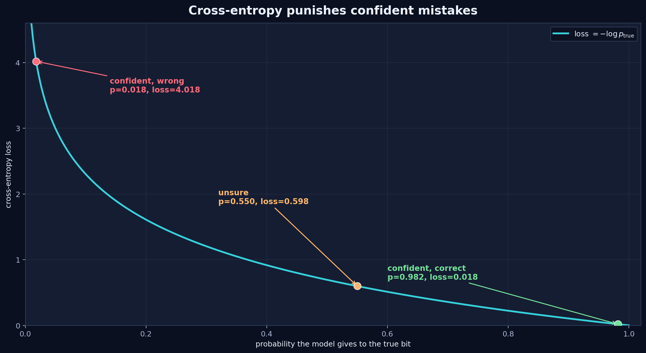
The curve is just \(-\log p_\text{true}\). When the model is right and sure the loss is near 0; when it is sure and wrong the loss explodes. Training simply slides each symbol along this curve toward the low end.
Next, why the nonlinearity is not optional. Save this as nonlinearity_demo.py:
import numpy as np
rng = np.random.default_rng(0)

x  = rng.normal(size=(1, 4))
W1 = rng.normal(size=(4, 8)); b1 = rng.normal(size=8)
W2 = rng.normal(size=(8, 2)); b2 = rng.normal(size=2)

# two linear layers with NO activation between them
linear_only = (x @ W1 + b1) @ W2 + b2

# the same thing collapses into ONE linear layer
W = W1 @ W2
b = b1 @ W2 + b2
single = x @ W + b

def silu(v):
    return v / (1.0 + np.exp(-v))

# with a nonlinearity the collapse no longer holds
with_silu = silu(x @ W1 + b1) @ W2 + b2

print("two linear layers  :", np.round(linear_only, 4))
print("one linear layer   :", np.round(single, 4))
print("max difference     :", np.abs(linear_only - single).max())
print("with SiLU (differs):", np.round(with_silu, 4))
python3 nonlinearity_demo.py
Expected output something like this:

The first two lines are identical up to rounding error (max difference is about 1e-16): two linear layers really are one linear layer. Only the SiLU line is different. Without it, the extra layer is wasted.
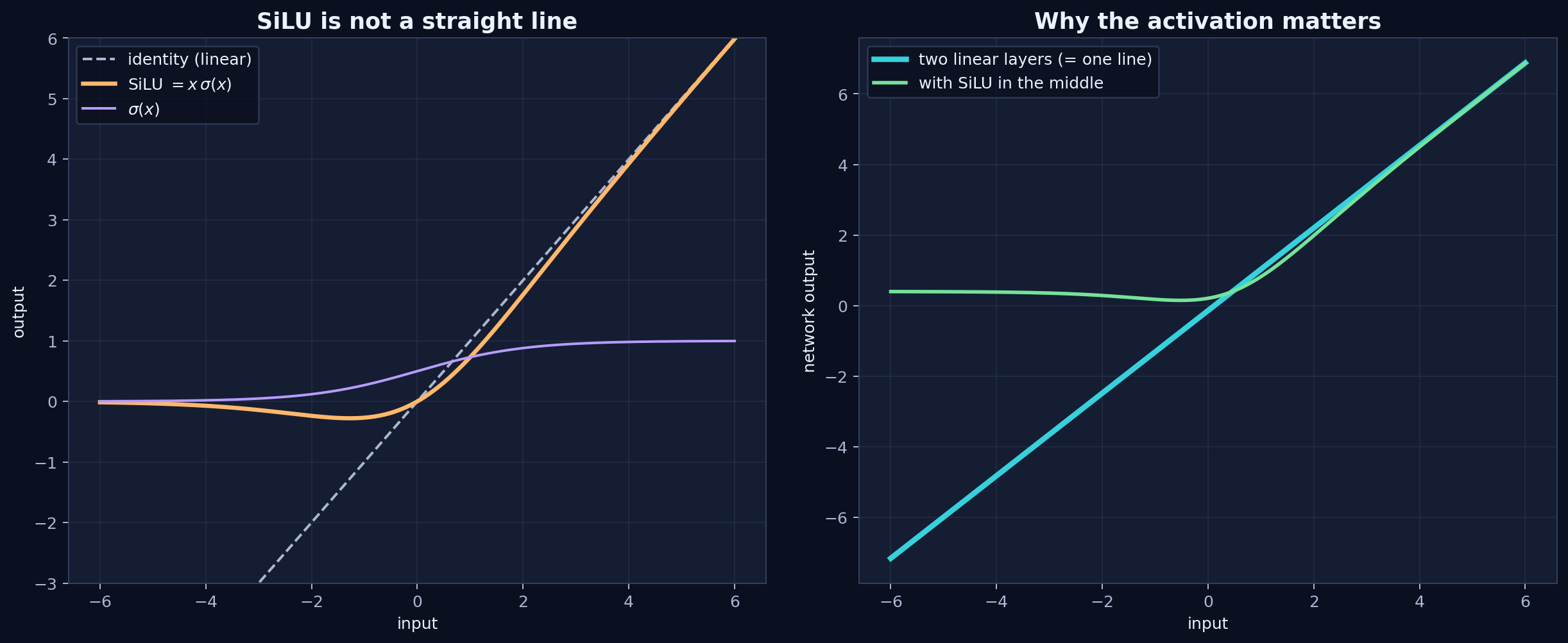
The left panel shows that SiLU bends where the plain identity does not. The right panel is the punchline: stack two Linear layers and the output is a straight line (cyan), no matter how many layers you add, until a nonlinearity (green) lets the network curve.
demo
Finally, watch a model actually learn a decision boundary. This is a one-feature logistic regression on a toy version of our problem: the feature is “energy at 2200 Hz minus energy at 1200 Hz”, and the model must learn that a positive value means bit 1. Save this as gd_demo.py:
import numpy as np
rng = np.random.default_rng(1)

# toy feature: (energy at 2200) - (energy at 1200); positive should mean bit 1
N = 4000
bits = rng.integers(0, 2, size=N)
feat = rng.normal(loc=np.where(bits == 1, 1.0, -1.0), scale=1.0)

def sigmoid(z):
    return 1.0 / (1.0 + np.exp(-z))

w, bias, lr = 0.0, 0.0, 0.5      # start with no decision at all
for step in range(1, 401):
    p = sigmoid(w * feat + bias)
    err = p - bits               # gradient of cross-entropy w.r.t. the logit
    w    -= lr * np.mean(err * feat)
    bias -= lr * np.mean(err)
    if step in (1, 50, 100, 200, 400):
        loss = -np.mean(bits*np.log(p+1e-9) + (1-bits)*np.log(1-p+1e-9))
        acc  = np.mean((p > 0.5) == bits)
        print(f"step={step:3d}  loss={loss:.4f}  acc={acc:.3f}  w={w:.3f}  bias={bias:.3f}")
python3 gd_demo.py
Expected output:
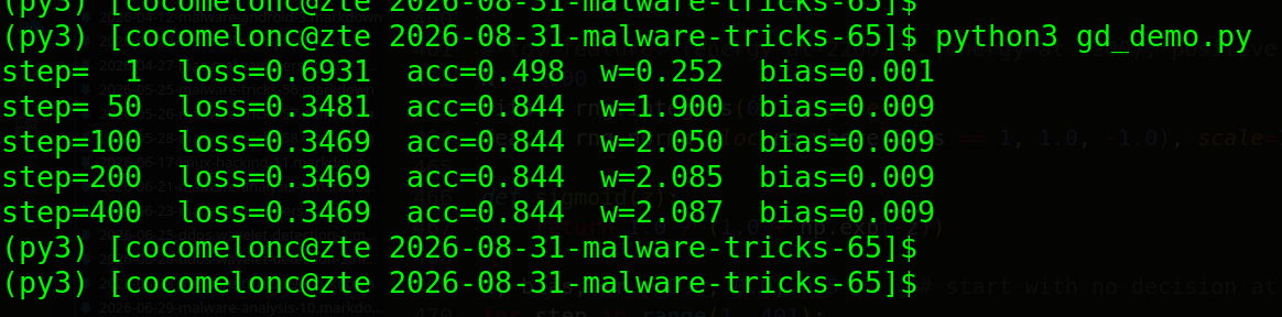
The weight w starts at 0 (no decision at all, about 50% accuracy) and gradient descent grows it until the model separates the two tones. The loss falls from 0.6931 to 0.3469, and accuracy rises to about 84%. DSPNet does the same thing, only in 405 dimensions and with a few hidden layers instead of one weight.
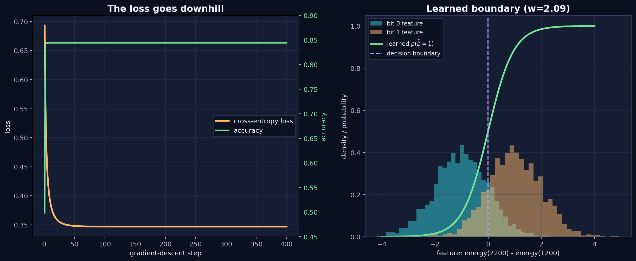
The left panel is the loss going downhill as the weight is updated. The right panel shows what the model actually learned: the two overlapping feature clouds (bit 0 and bit 1) and the fitted probability curve that splits them, with the decision boundary near 0. This is the same picture as the Goertzel rule, except the boundary was fitted from data instead of set by hand.
A small nuance. These demos are deliberately tiny so the math stays visible. The real training also uses mixed precision, AdamW, LayerNorm, and dropout, but the core loop is identical: turn logits into probabilities, measure the loss, follow the gradient downhill. If you understand the three scripts above, you already understand what the 1400-step loop on the L20 is doing.
training on NVIDIA L20
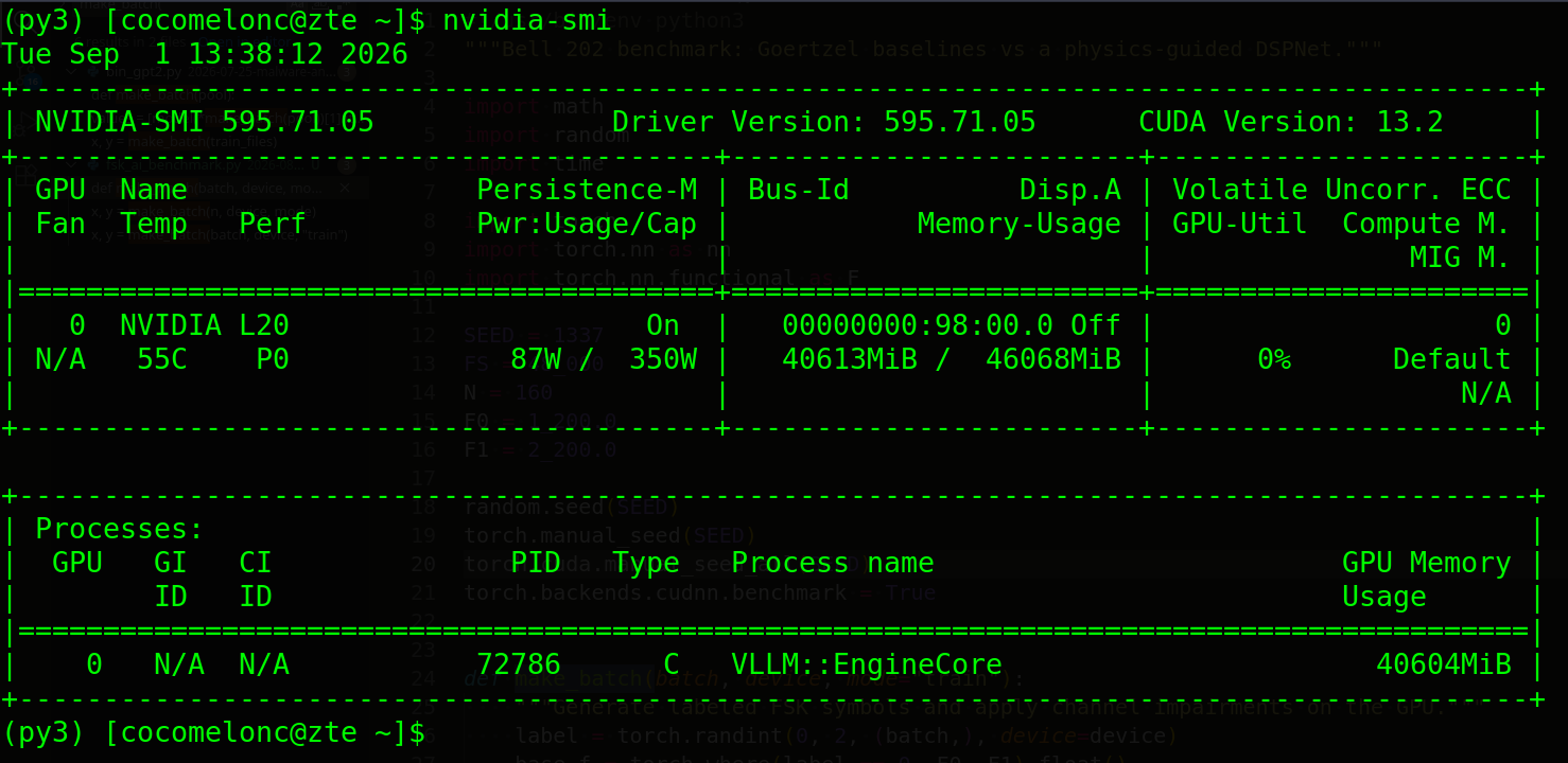
I used an NVIDIA L20 with 46 GB VRAM and PyTorch 2.6.0+cu124. The training loop is ordinary mixed-precision PyTorch:
device = torch.device("cuda")
model = DSPTinyDemod().to(device)
optimizer = torch.optim.AdamW(
    model.parameters(), lr=2e-3, weight_decay=1e-4
)
scaler = torch.amp.GradScaler("cuda")

for step in range(1, 1401):
    x, label = make_batch(2048, device, mode="train")
    optimizer.zero_grad(set_to_none=True)

    with torch.autocast(device_type="cuda", dtype=torch.float16):
        loss = F.cross_entropy(model(x), label)

    scaler.scale(loss).backward()
    scaler.step(optimizer)
    scaler.update()
Run the experiment:
python3 fsk_ai_benchmark.py
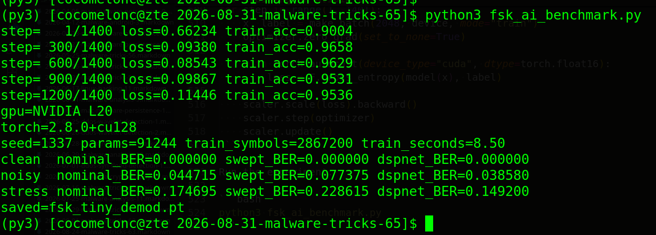
The complete run generated 2,867,200 training symbols on the fly and finished in ~8.50 seconds:
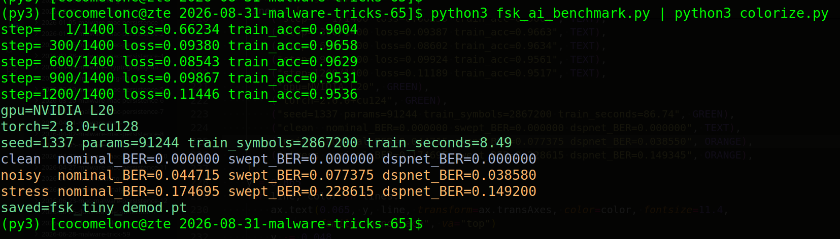
Colorized for demo:
results
Each row below contains 200,000 previously unseen symbols. All three receivers were evaluated on exactly the same batch within this run:
| test channel | nominal Goertzel BER | swept Goertzel BER | DSPNet BER |
|---|---|---|---|
| clean | 0.0000% |
0.0000% |
0.0000% |
| noisy | 4.4715% |
7.7375% |
3.8550% |
| stress | 17.4695% |
22.8615% |
14.9345% |
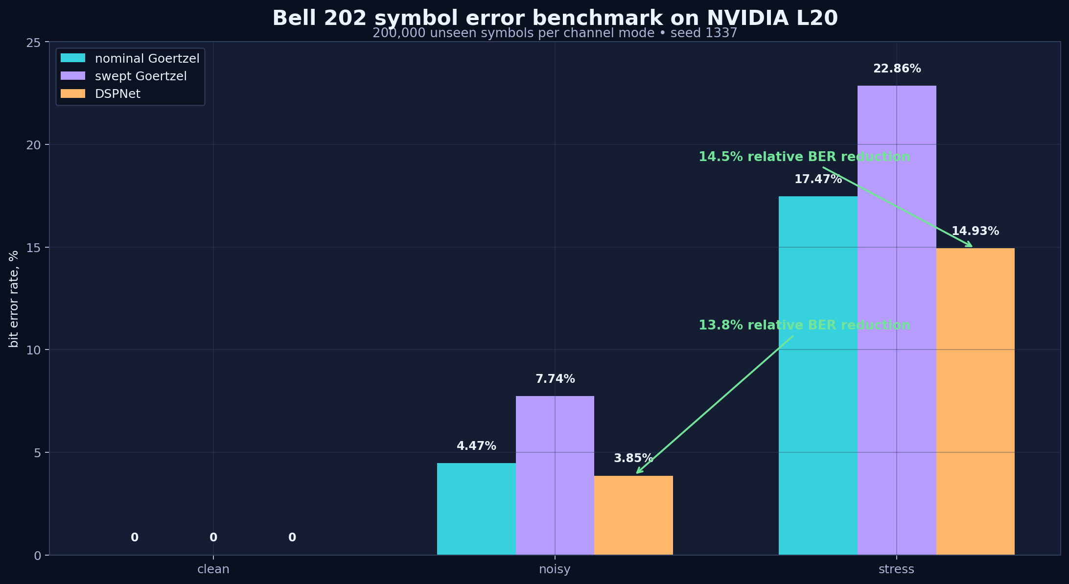
On the noisy set, DSPNet reduces BER by 0.6165 percentage points, or about 13.8% relative to nominal Goertzel. On the stress set, the reduction is 2.5350 points, or about 14.5% relative.
The wider swept-Goertzel baseline is an interesting warning. Searching more bins sounds safer, but a max-energy rule can lock onto a strong interfering tone. The learned head sees the shape across frequencies and across time, so it can sometimes distinguish a shifted FSK carrier from an unrelated narrow-band peak.
The swept baseline searches \(\pm175\) Hz around both carriers in 25 Hz steps and keeps the strongest bin. This is swept_goertzel_predict from fsk_ai_benchmark.py:
@torch.inference_mode()
def swept_goertzel_predict(x):
    """Stronger classical baseline: search +/- 175 Hz around both carriers."""
    device = x.device
    t = torch.arange(N, device=device).float() / FS
    offsets = torch.arange(-175.0, 176.0, 25.0, device=device)
    freqs = torch.cat([F0 + offsets, F1 + offsets])
    c = torch.cos(2 * math.pi * freqs[:, None] * t[None, :])
    s = torch.sin(2 * math.pi * freqs[:, None] * t[None, :])
    zc, zs = x[:, 0, :] @ c.T, x[:, 0, :] @ s.T
    power = zc.square() + zs.square()
    half = len(offsets)
    return (power[:, half:].amax(1) > power[:, :half].amax(1)).long()
The amax over the offsets is exactly the trap I described: a single strong interferer sitting near one carrier can win the maximum and flip the decided bit.
This is a modest improvement, not a magic replacement for DSP. On clean symbols all approaches are perfect, and the classical receiver requires no training data, model file, CUDA, or neural-network runtime.
All three numbers on each row come from a single loop that draws fresh symbols and scores every receiver on the very same batch, so the comparison is fair. This is evaluate from fsk_ai_benchmark.py:
@torch.inference_mode()
def evaluate(model, device, mode, total=200_000, batch=4096):
    model.eval()
    cnn_ok = classic_ok = swept_ok = count = 0
    while count < total:
        n = min(batch, total - count)
        x, y = make_batch(n, device, mode)
        cnn_ok += (model(x).argmax(1) == y).sum().item()
        classic_ok += (goertzel_predict(x) == y).sum().item()
        swept_ok += (swept_goertzel_predict(x) == y).sum().item()
        count += n
    return 1 - classic_ok / total, 1 - swept_ok / total, 1 - cnn_ok / total
Because make_batch builds one x and all three receivers score that same x on every iteration, any gap in the table is a property of the receiver, not luck in the random draw. Bit error rate is simply 1 - accuracy.
decode-only integration
The existing frame format can stay unchanged:
0xAA 0xAA 0xAA 0xAA 0x7E | uint16 length | payload | XOR checksum
The only replaced component is the one-symbol decision:
captured PCM
    -> timing/preamble search
    -> 160-sample symbol window
    -> fixed quadrature filter bank
    -> tiny neural head
    -> bit stream
    -> frame parser and checksum
    -> print recovered bytes
For the laboratory demo I will use a harmless payload:
PAYLOAD = b"MEOW FROM THE L20\n"
The receiver must reject a bad checksum and must never execute the recovered buffer. Later, the trained head can be exported to ONNX or rewritten as two small dense layers for a C receiver, while the filter-bank code remains ordinary DSP.
what this benchmark does not prove
The current result has several important limitations:
- symbols are already aligned; the model does not solve preamble acquisition or clock recovery;
- training and evaluation are synthetic, even though the stress ranges are harder;
- the channel generator is still one mathematical family, not a collection of real rooms, microphones, codecs, and speakers;
- BER is measured per symbol, not as complete-frame success;
- the model has only two outputs, so it must choose
0or1even for silence or ordinary music; - checksum and repetition detect failures but do not correct them.
That fourth point matters. A few percent BER is far too high for a long uncoded frame. A realistic next version needs forward error correction, interleaving, confidence thresholds, and an explicit third class such as NO_SYMBOL. The training set should also include clean music and speech as hard negative examples.
The proper next experiment is over-the-air data collection. Play randomized labeled frames through several speakers, record them with several microphones at different distances, keep entire devices or rooms out of the training set, and report frame success rate with confidence intervals. Until that experiment is complete, the current numbers are evidence about the simulator, not a claim about arbitrary real environments.
defensive perspective
The same architecture is arguably more useful for defenders. Replace the final classes with 1200, 2200, and NO_FSK, then scan audio streams for repeated modem-like structure. A useful detector should combine:
- persistent or alternating energy around the carrier bands;
- a repeated preamble and valid frame checksum;
- an audio-capturing process with unusual memory or process behavior;
- model confidence that remains high across consecutive symbol windows.
An ML score alone is not a verdict. Music, telemetry, accessibility software, and legitimate modem protocols can all create narrow-band patterns. Process context and a valid protocol structure provide the stronger signal.
conclusion
The experiment gave me a better result than a simple “let us add AI” story. The raw CNN lost to Goertzel. The physics-guided model improved only after I preserved the useful mathematical structure: quadrature filters, a local frequency grid, and multiple time windows.
The practical lesson is: use AI to combine good measurements, not to relearn obvious physics from a small dataset.
For the next revision I want to add real acoustic recordings, a NO_SYMBOL class, confidence calibration, forward error correction, and decode-only integration with the C receiver from the previous parts.
Bell 202 standard
Frequency-shift keying
Goertzel Algorithm
PyTorch
previous source repository
source code in github
This is a practical case for educational and authorized security research purposes only.
Thanks for your time, happy hacking and good bye!
PS. All drawings, screenshots, and benchmark results are mine.