Malware analysis: part 11. How to create your own mini-GPT for binary analysis.
﷽
Hello, cybersecurity enthusiasts and white hackers!
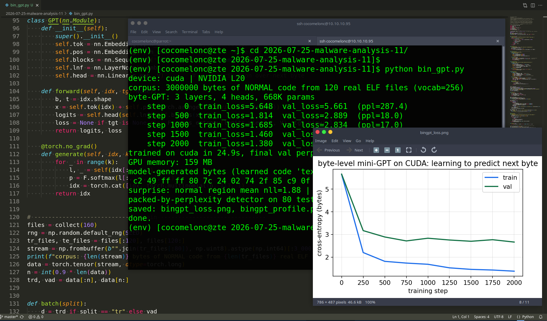
Everybody talks about GPT and large language models today. But a transformer is not magic - it is a small, understandable function trained with plain gradient descent. In this post we build our own mini-GPT completely from scratch in PyTorch, train it on raw bytes of real binaries, and turn it into a practical malware-analysis tool: a packing / encryption detector based on perplexity (how “surprised” the model is by the bytes it sees).
No black-box tools, no pretrained weights, no cloud API. Around 600K parameters, trained on a GPU in under half a minute. Everything is practice-oriented and reproducible.
the idea
A binary file is just a sequence of bytes. A GPT is a next-token predictor: given the previous bytes, it outputs a probability distribution over the next byte. If we train it only on normal machine code, it learns the “grammar” of real code - which byte usually follows e8 (a call), which patterns opcodes form, how padding looks.
Then we feed it new bytes and measure its surprise (the negative log-likelihood, a.k.a. perplexity):
normal code -> low surprise, the model predicts the next byte well;
packed / encrypted / compressed bytes -> high surprise, the model has no idea, because such bytes are close to random.
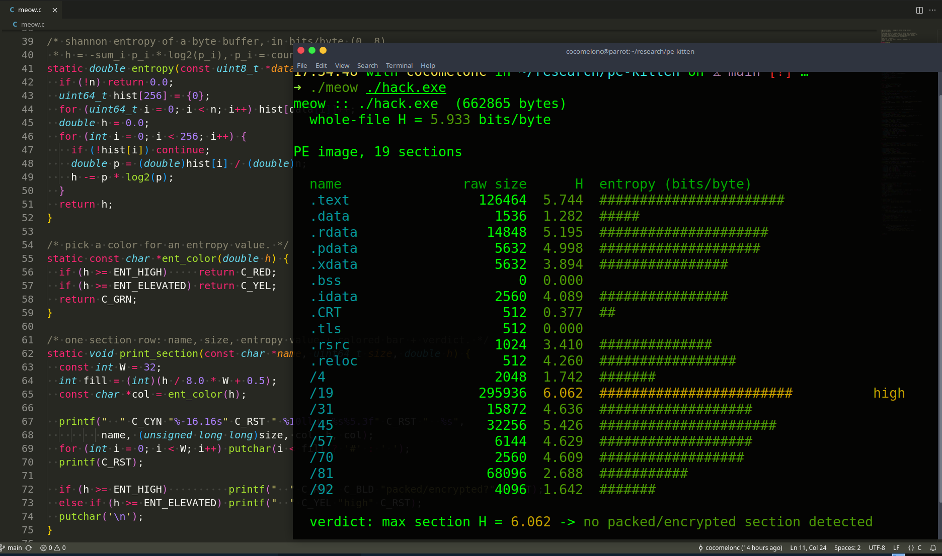
This is conceptually related to Shannon entropy from part 6, but it is smarter: entropy only counts byte frequencies, while the GPT models the order of bytes - the actual structure of code. That makes it a stronger signal for triage.
environment and data
You do not need a fancy setup - a Linux box with Python 3 is enough. A GPU is optional: this model is tiny and also trains on a plain CPU in a couple of minutes. If you have an NVIDIA GPU, the same script uses it automatically and trains in seconds.
We only need PyTorch, numpy and matplotlib. Start with a clean virtual environment:
python3 -m venv env && source env/bin/activate
pip install numpy matplotlib
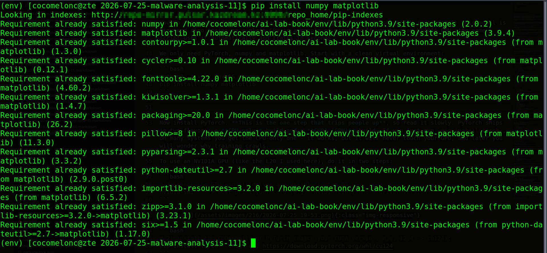
Now install PyTorch. This is the one step that trips people up, so read it slowly. PyTorch ships in two flavors: a CPU-only build and a CUDA (GPU) build. If you just run pip install torch, on many systems you get the CPU-only one - it works, but it will never touch your GPU, and later you will wonder why training crawls.
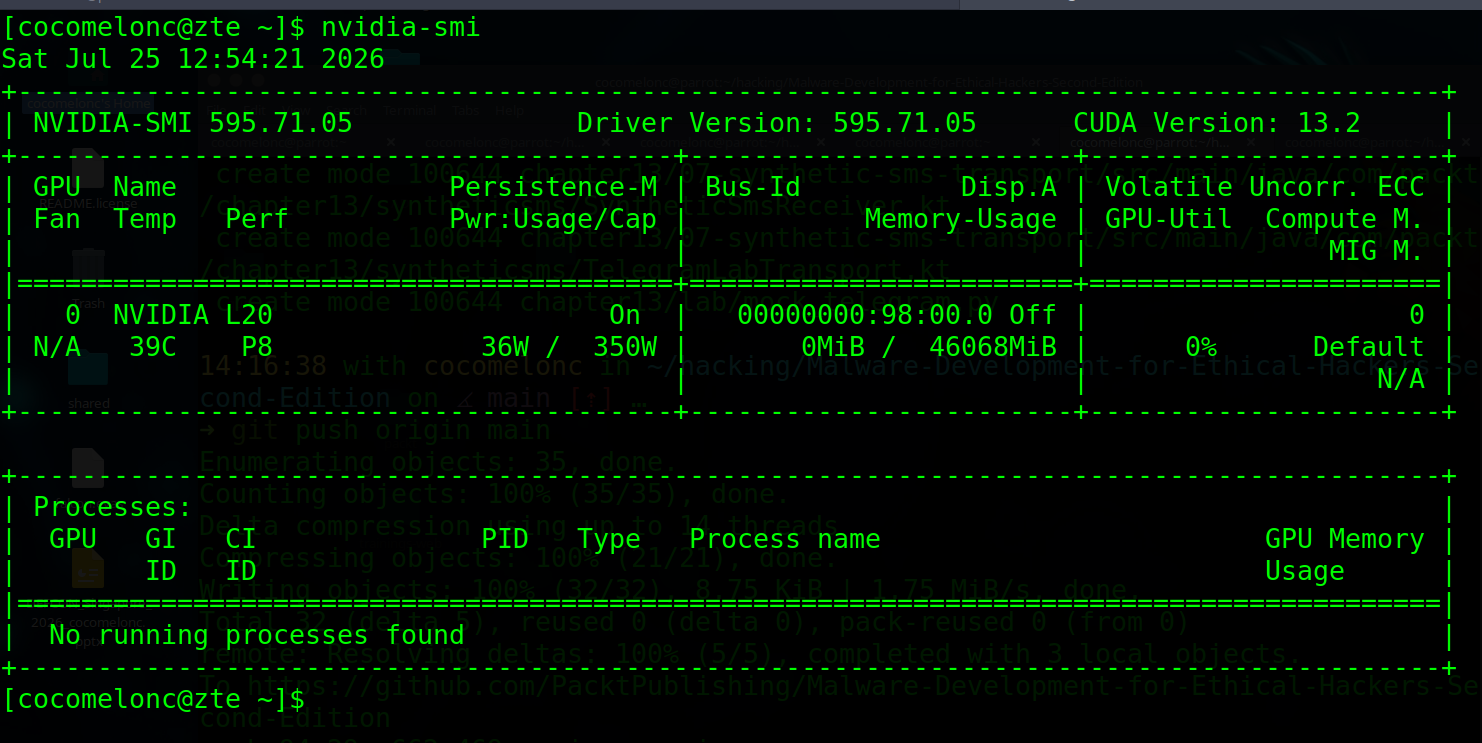
To use an NVIDIA GPU (like the L20 I used here), do it in two steps:
# 1) check the GPU and its driver are visible to the OS:
nvidia-smi     # must print your card (e.g. "NVIDIA L20") and a driver version
# 2) install the CUDA build of PyTorch (match your CUDA version, e.g. 12.4 -> cu124):
pip install torch --index-url https://download.pytorch.org/whl/cu124
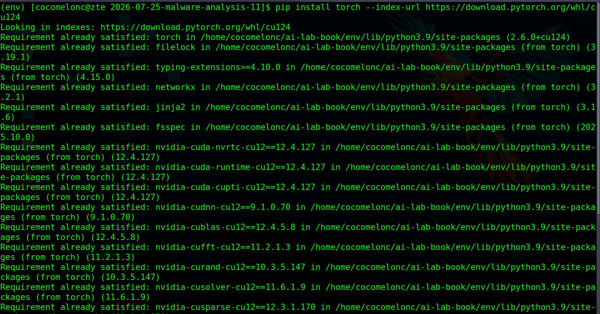
Copy the exact command for your CUDA version from the official page: pytorch.org/get-started. No NVIDIA GPU? Then just pip install torch and skip this - everything below still runs fine on CPU, only slower.
Now the important nuance - always verify that PyTorch really sees the GPU before you start training:
python3 -c "import torch; print(torch.cuda.is_available(), torch.cuda.get_device_name(0) if torch.cuda.is_available() else 'CPU')"
# GPU ready  ->  True NVIDIA L20
# CPU only   ->  False CPU

If it prints True and your GPU name - you are good. If it prints False but you do have an NVIDIA GPU, you almost certainly installed the CPU-only build: reinstall with the --index-url line above. Our script then picks the device automatically with a single line - dev = "cuda" if torch.cuda.is_available() else "cpu" - so the exact same code runs on your GPU or your laptop CPU with no changes.
practical example.
For training data we do not need any malware. We take real, legitimate ELF binaries from /usr/bin as our corpus of “normal code”. To get a packed sample for the detector, we simulate a packer the honest way - a small original header followed by a compressed body (real packers leave the same footprint: a low-entropy stub and a high-entropy compressed/encrypted body):
import os, glob, lzma, numpy as np

def collect(limit=160):
    out = []
    for p in sorted(glob.glob("/usr/bin/*")):
        try:
            if os.path.islink(p) or not (8000 < os.path.getsize(p) < 300000):
                continue
            b = open(p, "rb").read()
            if b[:4] == b"\x7fELF":
                out.append(b)
        except OSError:
            pass
        if len(out) >= limit:
            break
    return out

def pack_like(b, rng):                       # defensive packer simulation
    h = int(rng.integers(512, 4096))         # keep a small original header/stub
    body = b[h:]
    k = int(len(body) * rng.uniform(0.5, 1.0))
    return b[:h] + lzma.compress(body[:k], preset=int(rng.integers(1, 7))) + body[k:]
the model: a mini-GPT from scratch
Here is the whole transformer. It is a decoder-only GPT with causal self-attention - the same architecture as the big models, just tiny. Vocabulary is 256 (one token per byte).
# bin_gpt.py
# byte-level mini-GPT for binary analysis
# author: @cocomelonc
# https://cocomelonc.github.io/malware/2026/07/25/malware-analysis-11.html
import torch, torch.nn as nn
from torch.nn import functional as F

T, n_emb, n_head, n_layer, V = 64, 128, 4, 3, 256   # ctx, embed, heads, layers, vocab(bytes)

class Head(nn.Module):                        # one self-attention head
    def __init__(self, hs):
        super().__init__()
        self.k = nn.Linear(n_emb, hs, bias=False)
        self.q = nn.Linear(n_emb, hs, bias=False)
        self.v = nn.Linear(n_emb, hs, bias=False)
        self.register_buffer("mask", torch.tril(torch.ones(T, T)))
    def forward(self, x):
        b, t, c = x.shape
        att = (self.q(x) @ self.k(x).transpose(-2, -1)) * c ** -0.5   # scaled dot-product
        att = att.masked_fill(self.mask[:t, :t] == 0, float("-inf"))  # causal: no peeking ahead
        att = F.softmax(att, -1)
        return att @ self.v(x)

class Block(nn.Module):                        # attention + feed-forward with residuals
    def __init__(self):
        super().__init__()
        hs = n_emb // n_head
        self.h = nn.ModuleList([Head(hs) for _ in range(n_head)])
        self.proj = nn.Linear(n_emb, n_emb)
        self.ff = nn.Sequential(nn.Linear(n_emb, 4 * n_emb), nn.ReLU(), nn.Linear(4 * n_emb, n_emb))
        self.l1, self.l2 = nn.LayerNorm(n_emb), nn.LayerNorm(n_emb)
    def forward(self, x):
        x = x + self.proj(torch.cat([h(self.l1(x)) for h in self.h], -1))
        return x + self.ff(self.l2(x))

class GPT(nn.Module):
    def __init__(self):
        super().__init__()
        self.tok = nn.Embedding(V, n_emb)      # byte -> vector
        self.pos = nn.Embedding(T, n_emb)      # position -> vector
        self.blocks = nn.Sequential(*[Block() for _ in range(n_layer)])
        self.lnf = nn.LayerNorm(n_emb)
        self.head = nn.Linear(n_emb, V)        # -> distribution over next byte
    def forward(self, idx, tgt=None):
        b, t = idx.shape
        x = self.tok(idx) + self.pos(torch.arange(t, device=idx.device))
        logits = self.head(self.lnf(self.blocks(x)))
        loss = None if tgt is None else F.cross_entropy(logits.view(-1, V), tgt.view(-1))
        return logits, loss
    @torch.no_grad()
    def generate(self, idx, k):
        for _ in range(k):
            l, _ = self(idx[:, -T:])
            p = F.softmax(l[:, -1, :], -1)
            idx = torch.cat([idx, torch.multinomial(p, 1)], 1)
        return idx
That is it - self-attention, residual connections, layer norm, a feed-forward block, and a linear head. The famous transformer, about 60 lines.
training
The training loop is the same three steps you use for any neural net: forward, loss.backward(), opt.step(). We build one long byte stream from normal binaries and sample random windows.
import numpy as np, time, math

dev = "cuda" if torch.cuda.is_available() else "cpu"
files = collect(160); rng = np.random.default_rng(0)
tr_files, te_files = files[:120], files[120:]
stream = np.frombuffer(b"".join(tr_files[:80]), np.uint8).astype(np.int64)[:3_000_000]
data = torch.tensor(stream, dtype=torch.long)
n = int(0.9 * len(data)); trd, vad = data[:n], data[n:]

def batch(split):
    d = trd if split == "tr" else vad
    ix = torch.randint(len(d) - T, (64,))
    x = torch.stack([d[i:i+T]   for i in ix])
    y = torch.stack([d[i+1:i+T+1] for i in ix])
    return x.to(dev), y.to(dev)

torch.manual_seed(0); model = GPT().to(dev)
opt = torch.optim.AdamW(model.parameters(), 3e-3)
for s in range(2001):
    xb, yb = batch("tr")
    _, loss = model(xb, yb)
    opt.zero_grad(); loss.backward(); opt.step()
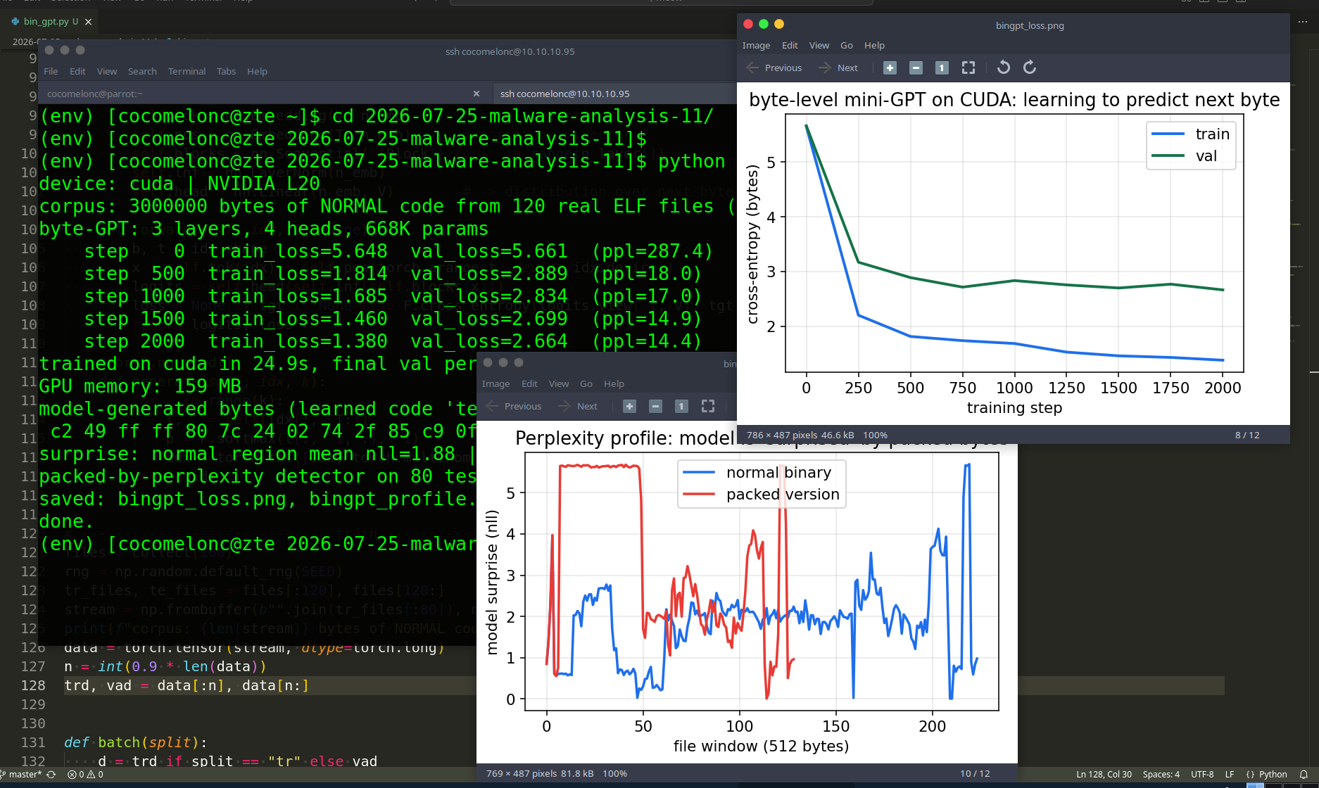
Let’s run it. I trained on an NVIDIA L20, but the exact same script runs on any machine (it just falls back to CPU):
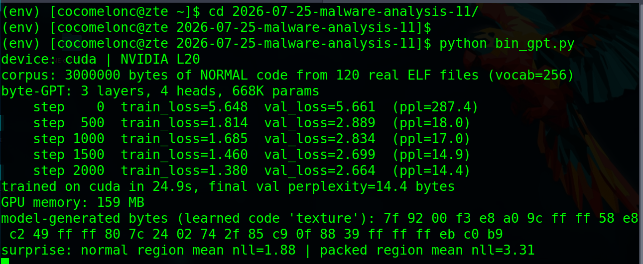
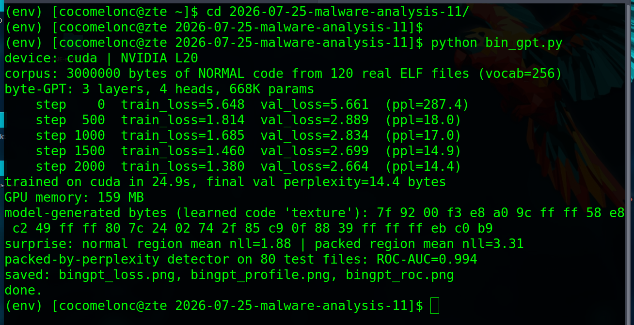
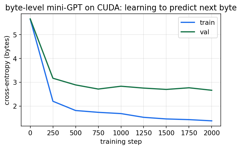
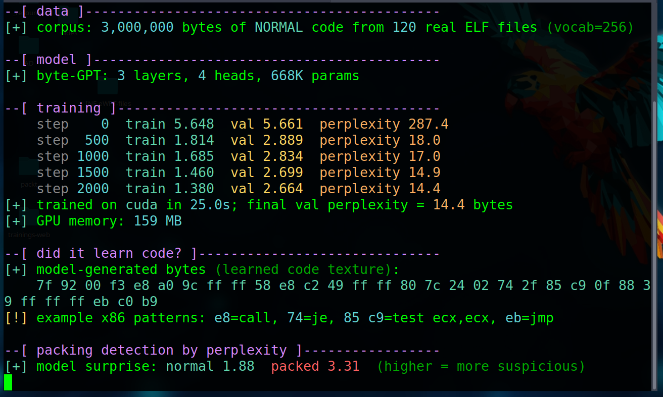
The validation perplexity drops from 287 down to ~14 bytes in about 25 seconds. Perplexity 14 means that, on average, the model narrows the next byte down to roughly 14 likely candidates out of 256 - it has genuinely learned the structure of machine code.
did it actually learn code?
Let’s ask the model to generate bytes from scratch and look at them as hex:
seed = torch.tensor([[0x7f]], device=dev)
print(model.generate(seed, 64)[0].cpu().numpy().astype("uint8").tobytes().hex(" "))

7f 92 00 f3 e8 a0 9c ff ff 58 e8 c2 49 ff ff 80 7c 24 02 74 2f 85 c9 0f 88 39 ff ff ff eb c0 b9
This is not random noise - it looks like real x86. We can literally read opcodes in it: e8 .. ff ff is a call rel32, 74 2f is je, 85 c9 is test ecx, ecx, 0f 88 is js, eb is a short jmp, b9 is mov ecx, imm32. Our tiny model learned the texture of compiled code purely from bytes, with no disassembler and no labels.
The model learns the distribution of normal data:
\[p\left(x_t \mid x_{t-T}, \ldots, x_{t-1}\right)\]where, \(x_t\) - this is the byte of the binary file at position \(t\).
and the unusualness of the byte is estimated as:
\[\mathrm{NLL}_t = -\log p\left(x_t \mid x_{<t}\right)\]the payoff: packing detection by perplexity
Now the malware-analysis part. We measure how surprised the trained model is per file window. Normal code = low surprise; packed/encrypted body = high surprise.
@torch.no_grad()
def nll(byte_ints):                            # per-position negative log-likelihood
    model.eval()
    x = torch.tensor(byte_ints, dtype=torch.long, device=dev); out = []
    for i in range(0, len(x) - 1, T):
        ch = x[i:i+T+1]
        if len(ch) < 2: break
        lg, _ = model(ch[:-1].unsqueeze(0))
        lp = F.log_softmax(lg[0], -1); tg = ch[1:]
        out.append((-lp[torch.arange(len(tg)), tg]).cpu().numpy())
    return np.concatenate(out)

def winavg(a, w=512):                           # average surprise per 512-byte window
    return np.array([a[i:i+w].mean() for i in range(0, len(a) - w + 1, w)])
Plotting the per-window surprise for one normal binary and its packed version makes the effect obvious:
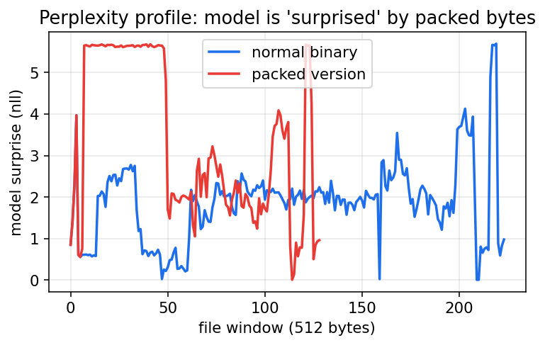
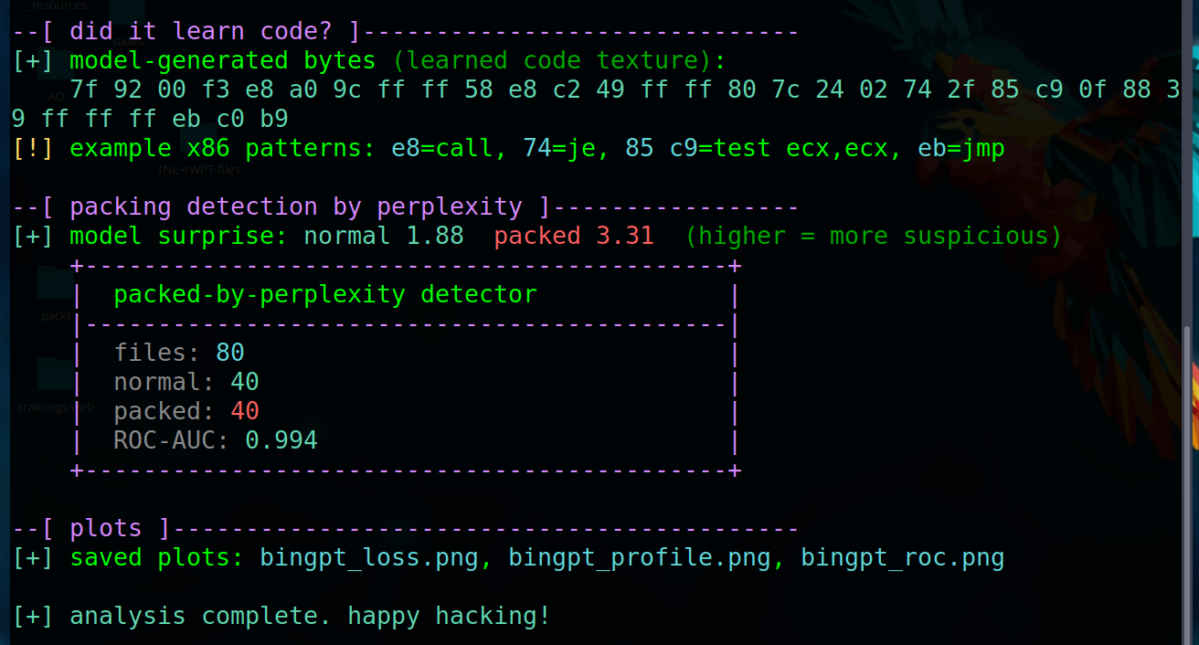
The blue line (normal binary) stays low in the code sections. The red line (packed version) has a huge plateau of high surprise exactly where the compressed body sits - the model screams “I have never seen bytes like this”. Average surprise was 1.88 on normal regions vs 3.31 on packed regions.
Turned into a simple detector - mean surprise over the first 60 KB of each file - and evaluated on 80 held-out files (each in a normal and a packed variant):
def score(b):
    return nll(np.frombuffer(b[:60000], np.uint8).astype(np.int64)).mean()
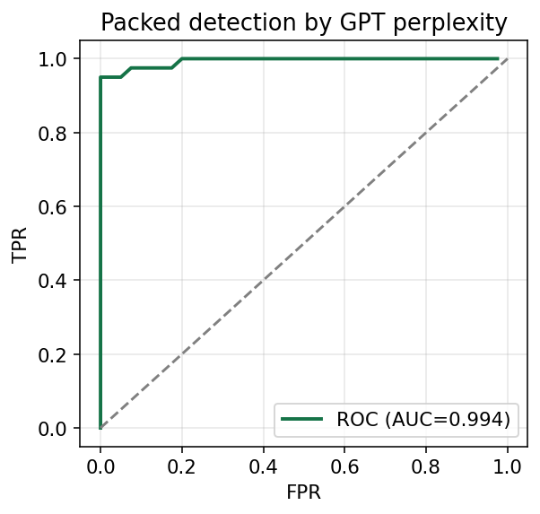
ROC-AUC = 0.994. A 600K-parameter transformer we wrote by hand, trained for 25 seconds, separates packed from unpacked binaries almost perfectly - and, unlike a plain entropy threshold, it reacts to unusual code order, not just byte frequency.
I also added some colors to final script:
practical example 2: making the experiment stricter
The first example was intentionally tutorial-first: one short script, one continuous byte stream, one synthetic task, and enough code to expose the complete pipeline without hiding it behind ML frameworks. That is useful for learning, but it is not yet a strong claim about detector effectiveness. So I wrote a second script, bin_gpt2.py, which keeps the same tiny model and fixes the experimental design instead of making the network larger.
First, scaled dot-product attention must use the query/key width of one head. In the first minimal version, c is the full embedding width (128); the correct scale is based on head_size = 128 / 4 = 32:
class Head(nn.Module):
    def __init__(self, head_size):
        super().__init__()
        self.k = nn.Linear(N_EMB, head_size, bias=False)
        self.q = nn.Linear(N_EMB, head_size, bias=False)
        self.v = nn.Linear(N_EMB, head_size, bias=False)
        self.scale = head_size ** -0.5

    def forward(self, x):
        att = (self.q(x) @ self.k(x).transpose(-2, -1)) * self.scale
The difference is 32^-0.5 = 0.1768 instead of 128^-0.5 = 0.0884. The old model still trained, but its attention logits were unnecessarily compressed and the softmax distribution was smoother than standard scaled attention requires.
The second version also separates the terminology. NLL is the mean negative log-likelihood in nats per predicted byte token:
\[\mathrm{NLL} = -\frac{1}{N}\sum_{t=1}^{N}\log p(x_t\mid x_{<t})\]Perplexity is exp(NLL) and is dimensionless. Therefore the detector uses mean NLL as its anomaly score; perplexity is reported only as an easier-to-read training metric. It is not measured in bytes.
The data split is now performed by file. The script parses each ELF section table and extracts only .text, then creates three disjoint sets:
train_files      = files[:100]
validation_files = files[100:120]
test_files       = files[120:160]
This means validation windows cannot come from a binary already present in training. It also means the model is trained on executable sections rather than ELF headers, symbol strings, resources, and other file data. A .text section can still contain compiler padding or embedded constants, so “machine code only” is an approximation, but it is much closer to the research question.
During scoring, contexts overlap with a stride of 32. Every target byte is counted once, while later predictions retain up to 64 preceding bytes. This removes the artificial context reset at every non-overlapping 64-byte boundary. Byte generation is not used as quantitative proof: readable opcodes are an interesting sanity check, but only held-out likelihood and downstream metrics measure the model.
Finally, the same 40 held-out ELF binaries are scored twice: once in original form and once after the synthetic packing transformation. The exact statement is therefore 40 unique base binaries producing 80 evaluation instances: 40 original and 40 synthetically packed variants. This is a paired synthetic benchmark, not evidence that the detector generalizes to all real packers or malware.
Full second script (bin_gpt2.py):
#!/usr/bin/env python3
# bin_gpt2.py
# stricter byte-GPT packed-code benchmark:
# file-level splits, ELF .text only, corrected attention scaling,
# overlapping context, entropy baseline, and paired confidence intervals.
# author: @cocomelonc
# https://cocomelonc.github.io/malware/2026/07/25/malware-analysis-11.html
#
# run:  python3 bin_gpt2.py
# test: python3 bin_gpt2.py --smoke
# deps: pip install torch numpy matplotlib

import glob
import lzma
import math
import os
import struct
import sys
import time

import matplotlib
matplotlib.use("Agg")
import matplotlib.pyplot as plt
import numpy as np
import torch
import torch.nn as nn
from torch.nn import functional as F


# --------------------------- terminal colors ---------------------------
_COLOR = (
    os.environ.get("FORCE_COLOR") == "1"
    or (sys.stdout.isatty() and "NO_COLOR" not in os.environ)
)


def color(code, text):
    return f"\033[{code}m{text}\033[0m" if _COLOR else text


def info(text):
    print(f"{color('1;38;5;75', '[*]')} {text}")


def ok(text):
    print(f"{color('1;38;5;79', '[+]')} {text}")


def section(text):
    print(f"\n{color('1;38;5;177', f'--[ {text} ]' + '-' * 42)}")


# ------------------------------- config -------------------------------
SMOKE = "--smoke" in sys.argv
T, N_EMB, N_HEAD, N_LAYER, V = 64, 128, 4, 3, 256
HEAD_SIZE = N_EMB // N_HEAD
STEPS = 2 if SMOKE else 2000
BATCH_SIZE = 8 if SMOKE else 64
SCORE_BYTES = 4096 if SMOKE else 32768
STRIDE = 32
SEED = 0
DEVICE = "cuda" if torch.cuda.is_available() else "cpu"

torch.manual_seed(SEED)
if torch.cuda.is_available():
    torch.cuda.manual_seed_all(SEED)
train_rng = np.random.default_rng(SEED)
pack_rng = np.random.default_rng(SEED + 1)


# ------------------------------- data ---------------------------------
def elf_text(path):
    """Return the .text section from a little-endian ELF32/ELF64 file."""
    try:
        data = open(path, "rb").read()
    except OSError:
        return None
    if data[:4] != b"\x7fELF" or len(data) < 64 or data[5] != 1:
        return None

    elf_class = data[4]
    if elf_class == 2:
        shoff = struct.unpack_from("<Q", data, 40)[0]
        shentsize, shnum, shstrndx = struct.unpack_from("<HHH", data, 58)
        shfmt = "<IIQQQQIIQQ"
    elif elf_class == 1:
        shoff = struct.unpack_from("<I", data, 32)[0]
        shentsize, shnum, shstrndx = struct.unpack_from("<HHH", data, 46)
        shfmt = "<IIIIIIIIII"
    else:
        return None

    expected = struct.calcsize(shfmt)
    if (
        shentsize < expected
        or shnum == 0
        or shstrndx >= shnum
        or shoff + shentsize * shnum > len(data)
    ):
        return None

    sections = [
        struct.unpack_from(shfmt, data, shoff + i * shentsize)
        for i in range(shnum)
    ]
    names_header = sections[shstrndx]
    names_offset, names_size = names_header[4], names_header[5]
    names = data[names_offset:names_offset + names_size]

    for header in sections:
        name_offset, section_type = header[0], header[1]
        end = names.find(b"\0", name_offset)
        if end < 0:
            continue
        name = names[name_offset:end]
        offset, size = header[4], header[5]
        if name == b".text" and section_type == 1:
            section = data[offset:offset + size]
            return section if len(section) >= T + 2 else None
    return None


def collect(limit):
    """Collect independent machine-code sections, preserving file identity."""
    files = []
    for path in sorted(glob.glob("/usr/bin/*")):
        if os.path.islink(path):
            continue
        text = elf_text(path)
        if text is not None and len(text) >= SCORE_BYTES:
            files.append((path, text))
        if len(files) == limit:
            break
    return files


def pack_like(code, rng):
    """Synthetic packed-code variant: small stub plus compressed code body."""
    stub = min(1024, max(256, len(code) // 20))
    body = code[stub:]
    packed_size = int(len(body) * rng.uniform(0.65, 1.0))
    preset = int(rng.integers(1, 7))
    return code[:stub] + lzma.compress(body[:packed_size], preset=preset) + body[packed_size:]


# ------------------------------- model --------------------------------
class Head(nn.Module):
    """One causal attention head, scaled by its own query/key width."""

    def __init__(self, head_size):
        super().__init__()
        self.k = nn.Linear(N_EMB, head_size, bias=False)
        self.q = nn.Linear(N_EMB, head_size, bias=False)
        self.v = nn.Linear(N_EMB, head_size, bias=False)
        self.scale = head_size ** -0.5
        self.register_buffer(
            "mask",
            torch.tril(torch.ones(T, T, dtype=torch.bool)),
        )

    def forward(self, x):
        _, length, _ = x.shape
        attention = (
            self.q(x) @ self.k(x).transpose(-2, -1)
        ) * self.scale
        attention = attention.masked_fill(
            ~self.mask[:length, :length],
            float("-inf"),
        )
        return F.softmax(attention, dim=-1) @ self.v(x)


class Block(nn.Module):
    def __init__(self):
        super().__init__()
        self.heads = nn.ModuleList(
            [Head(HEAD_SIZE) for _ in range(N_HEAD)]
        )
        self.projection = nn.Linear(N_EMB, N_EMB)
        self.feed_forward = nn.Sequential(
            nn.Linear(N_EMB, 4 * N_EMB),
            nn.ReLU(),
            nn.Linear(4 * N_EMB, N_EMB),
        )
        self.norm1 = nn.LayerNorm(N_EMB)
        self.norm2 = nn.LayerNorm(N_EMB)

    def forward(self, x):
        normalized = self.norm1(x)
        joined = torch.cat([head(normalized) for head in self.heads], dim=-1)
        x = x + self.projection(joined)
        return x + self.feed_forward(self.norm2(x))


class GPT(nn.Module):
    def __init__(self):
        super().__init__()
        self.token_embedding = nn.Embedding(V, N_EMB)
        self.position_embedding = nn.Embedding(T, N_EMB)
        self.blocks = nn.Sequential(*[Block() for _ in range(N_LAYER)])
        self.final_norm = nn.LayerNorm(N_EMB)
        self.output = nn.Linear(N_EMB, V)

    def forward(self, indices, targets=None):
        _, length = indices.shape
        positions = torch.arange(length, device=indices.device)
        x = self.token_embedding(indices) + self.position_embedding(positions)
        logits = self.output(self.final_norm(self.blocks(x)))
        loss = None
        if targets is not None:
            loss = F.cross_entropy(
                logits.reshape(-1, V),
                targets.reshape(-1),
            )
        return logits, loss


def make_batch(pool):
    """Sample windows from distinct files; never concatenate file boundaries."""
    windows = []
    for _ in range(BATCH_SIZE):
        _, code = pool[int(train_rng.integers(len(pool)))]
        start = int(train_rng.integers(0, len(code) - T - 1))
        windows.append(np.frombuffer(code[start:start + T + 1], np.uint8))
    batch = torch.tensor(
        np.stack(windows).astype(np.int64),
        dtype=torch.long,
        device=DEVICE,
    )
    return batch[:, :-1], batch[:, 1:]


@torch.no_grad()
def estimate_nll(model, pool, batches=15):
    """Mean next-byte NLL in nats/token; perplexity is exp(NLL)."""
    model.eval()
    values = [model(*make_batch(pool))[1].item() for _ in range(batches)]
    return float(np.mean(values))


@torch.no_grad()
def sliding_nll(model, code):
    """Score each target once while retaining overlapping left context."""
    byte_values = np.frombuffer(code[:SCORE_BYTES], np.uint8).astype(np.int64)
    if len(byte_values) < 2:
        return np.empty(0)

    if len(byte_values) <= T + 1:
        x = torch.tensor(byte_values, device=DEVICE).unsqueeze(0)
        logits, _ = model(x[:, :-1])
        targets = x[:, 1:]
        losses = F.cross_entropy(
            logits.reshape(-1, V),
            targets.reshape(-1),
            reduction="none",
        )
        return losses.cpu().numpy()

    last_start = len(byte_values) - T - 1
    starts = list(range(0, last_start + 1, STRIDE))
    if starts[-1] != last_start:
        starts.append(last_start)

    covered_target = 0
    keep_counts = []
    windows = []
    for start in starts:
        windows.append(byte_values[start:start + T + 1])
        end_target = start + T
        keep_counts.append(end_target - covered_target)
        covered_target = end_target

    output = []
    for base in range(0, len(windows), 128):
        chunk = torch.tensor(
            np.stack(windows[base:base + 128]),
            dtype=torch.long,
            device=DEVICE,
        )
        logits, _ = model(chunk[:, :-1])
        losses = F.cross_entropy(
            logits.reshape(-1, V),
            chunk[:, 1:].reshape(-1),
            reduction="none",
        ).reshape(len(chunk), T)
        for row, keep in zip(
            losses,
            keep_counts[base:base + len(chunk)],
        ):
            output.append(row[-keep:].cpu().numpy())
    return np.concatenate(output)


# ------------------------------ metrics -------------------------------
def shannon_entropy(code):
    values = np.frombuffer(code[:SCORE_BYTES], np.uint8)
    counts = np.bincount(values, minlength=V).astype(float)
    probabilities = counts[counts > 0] / max(len(values), 1)
    return float(-(probabilities * np.log2(probabilities)).sum())


def auc_score(normal, packed):
    """Probability that a random positive score exceeds a negative score."""
    differences = packed[:, None] - normal[None, :]
    return float(
        (np.count_nonzero(differences > 0)
         + 0.5 * np.count_nonzero(differences == 0))
        / differences.size
    )


def roc_curve(normal, packed):
    scores = np.concatenate([normal, packed])
    labels = np.concatenate([
        np.zeros(len(normal), dtype=int),
        np.ones(len(packed), dtype=int),
    ])
    thresholds = np.r_[
        np.inf,
        np.sort(np.unique(scores))[::-1],
        -np.inf,
    ]
    tpr, fpr = [], []
    for threshold in thresholds:
        predicted = scores >= threshold
        tpr.append(np.mean(predicted[labels == 1]))
        fpr.append(np.mean(predicted[labels == 0]))
    return np.asarray(fpr), np.asarray(tpr)


def fpr_at_tpr(normal, packed, target=0.95):
    fpr, tpr = roc_curve(normal, packed)
    eligible = fpr[tpr >= target]
    return float(eligible.min()) if len(eligible) else 1.0


def paired_auc_ci(normal, packed, rounds):
    """Bootstrap base files, keeping original/packed pairs together."""
    rng = np.random.default_rng(SEED + 2)
    estimates = []
    for _ in range(rounds):
        indices = rng.integers(0, len(normal), len(normal))
        estimates.append(auc_score(normal[indices], packed[indices]))
    return tuple(np.quantile(estimates, [0.025, 0.975]))


# ------------------------------- run ----------------------------------
section("file-level dataset")
limit = 40 if SMOKE else 160
files = collect(limit)
if len(files) != limit:
    raise RuntimeError(
        f"need {limit} ELF files with usable .text sections, found {len(files)}"
    )

if SMOKE:
    train_files, validation_files, test_files = (
        files[:25],
        files[25:30],
        files[30:],
    )
else:
    train_files, validation_files, test_files = (
        files[:100],
        files[100:120],
        files[120:],
    )

ok(
    f"train={len(train_files)}, validation={len(validation_files)}, "
    f"test={len(test_files)} unique ELF files; .text only"
)
info(f"device={DEVICE}, head_size={HEAD_SIZE}, scale={HEAD_SIZE ** -0.5:.4f}")

section("training")
model = GPT().to(DEVICE)
optimizer = torch.optim.AdamW(model.parameters(), lr=3e-3)
start_time = time.time()
for step in range(STEPS + 1):
    if step % (1 if SMOKE else 500) == 0:
        train_nll = estimate_nll(model, train_files, 2 if SMOKE else 15)
        validation_nll = estimate_nll(
            model,
            validation_files,
            2 if SMOKE else 15,
        )
        print(
            f"step={step:4d} "
            f"train_NLL={train_nll:.3f} "
            f"validation_NLL={validation_nll:.3f} "
            f"validation_PPL={math.exp(validation_nll):.2f}"
        )
    x, y = make_batch(train_files)
    _, loss = model(x, y)
    optimizer.zero_grad()
    loss.backward()
    optimizer.step()

ok(f"training completed in {time.time() - start_time:.1f}s")

section("paired synthetic benchmark")
model.eval()
original = [code for _, code in test_files]
packed = [pack_like(code, pack_rng) for code in original]

gpt_normal = np.asarray([sliding_nll(model, code).mean() for code in original])
gpt_packed = np.asarray([sliding_nll(model, code).mean() for code in packed])
entropy_normal = np.asarray([shannon_entropy(code) for code in original])
entropy_packed = np.asarray([shannon_entropy(code) for code in packed])

bootstrap_rounds = 50 if SMOKE else 1000
gpt_auc = auc_score(gpt_normal, gpt_packed)
entropy_auc = auc_score(entropy_normal, entropy_packed)
gpt_ci = paired_auc_ci(gpt_normal, gpt_packed, bootstrap_rounds)
entropy_ci = paired_auc_ci(
    entropy_normal,
    entropy_packed,
    bootstrap_rounds,
)

print(
    f"base binaries={len(test_files)}, evaluation instances={2 * len(test_files)}"
)
print(
    f"GPT mean NLL: AUC={gpt_auc:.3f} "
    f"95% CI=[{gpt_ci[0]:.3f}, {gpt_ci[1]:.3f}] "
    f"FPR@95%TPR={fpr_at_tpr(gpt_normal, gpt_packed):.3f}"
)
print(
    f"entropy bits/byte: AUC={entropy_auc:.3f} "
    f"95% CI=[{entropy_ci[0]:.3f}, {entropy_ci[1]:.3f}] "
    f"FPR@95%TPR={fpr_at_tpr(entropy_normal, entropy_packed):.3f}"
)

section("plot")
gpt_fpr, gpt_tpr = roc_curve(gpt_normal, gpt_packed)
ent_fpr, ent_tpr = roc_curve(entropy_normal, entropy_packed)
figure, axes = plt.subplots(1, 2, figsize=(9, 3.8))

axes[0].plot(gpt_fpr, gpt_tpr, lw=2, label=f"GPT NLL ({gpt_auc:.3f})")
axes[0].plot(ent_fpr, ent_tpr, lw=2, label=f"entropy ({entropy_auc:.3f})")
axes[0].plot([0, 1], [0, 1], "--", color="gray")
axes[0].set(
    xlabel="false-positive rate",
    ylabel="true-positive rate",
    title="Synthetic packed-code ROC",
)
axes[0].legend(loc="lower right")
axes[0].grid(alpha=0.3)

values = [gpt_auc, entropy_auc]
low = [
    max(0.0, gpt_auc - gpt_ci[0]),
    max(0.0, entropy_auc - entropy_ci[0]),
]
high = [
    max(0.0, gpt_ci[1] - gpt_auc),
    max(0.0, entropy_ci[1] - entropy_auc),
]
axes[1].bar(["GPT NLL", "entropy"], values, color=["#4c78a8", "#f58518"])
axes[1].errorbar(
    [0, 1],
    values,
    yerr=[low, high],
    fmt="none",
    color="black",
    capsize=4,
)
axes[1].set_ylim(0.45, 1.02)
axes[1].set_ylabel("ROC-AUC")
axes[1].set_title("Paired bootstrap 95% CI")
axes[1].grid(axis="y", alpha=0.3)

figure.tight_layout()
figure.savefig("bingpt2_benchmark.png", dpi=140)
ok("saved bingpt2_benchmark.png")
print(f"\n{color('1;38;5;79', '[+] analysis complete. happy hacking!')}\n")
demo 2
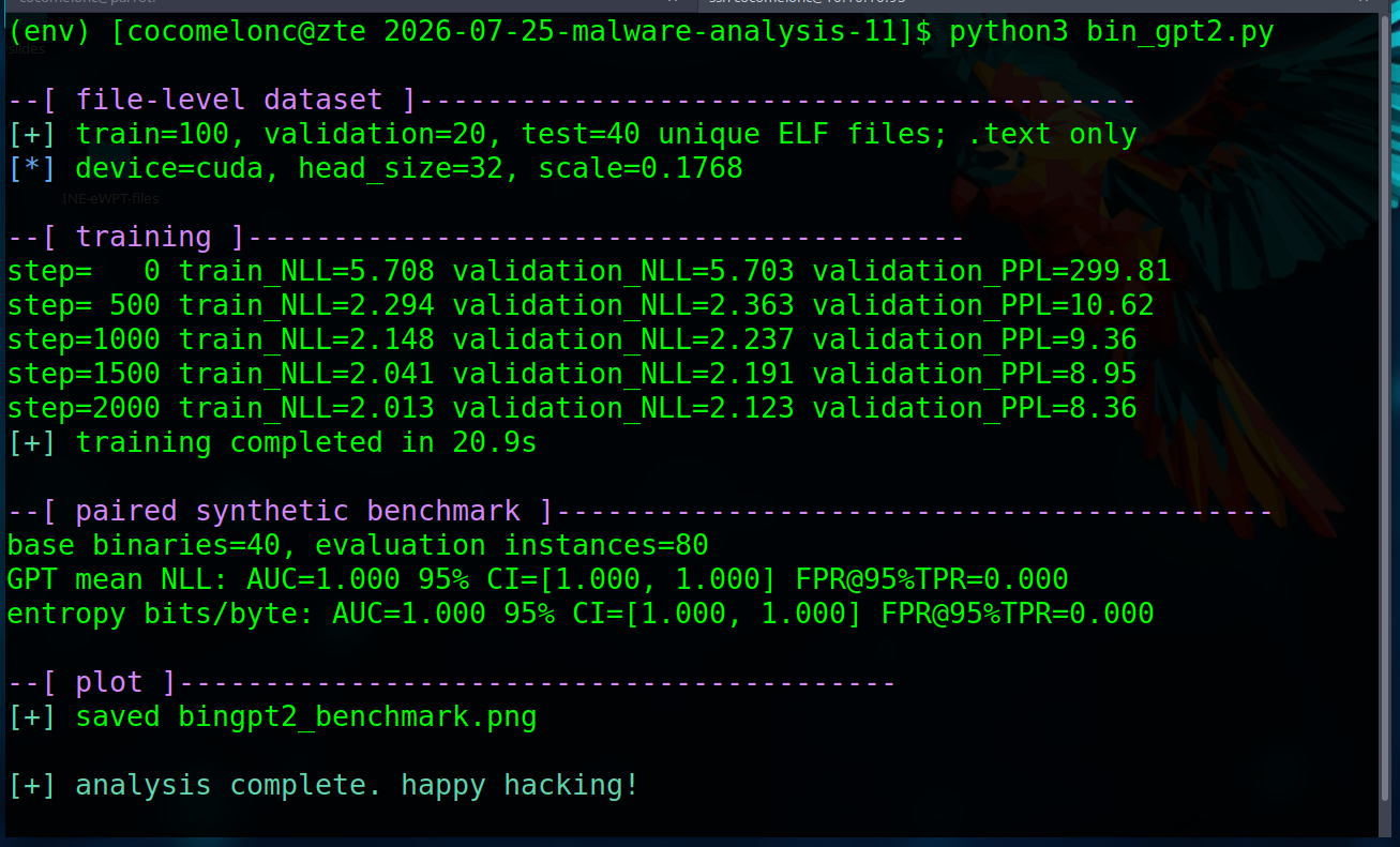
Run the stricter experiment exactly like the first one:
python3 bin_gpt2.py
For a quick CPU pipeline check without waiting for full training:
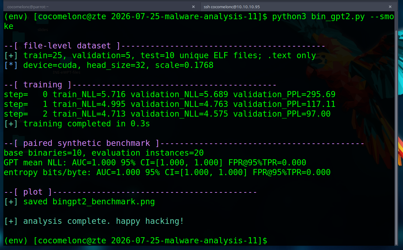
python3 bin_gpt2.py --smoke
The result now compares the GPT score with a Shannon entropy baseline on exactly the same files and bytes:
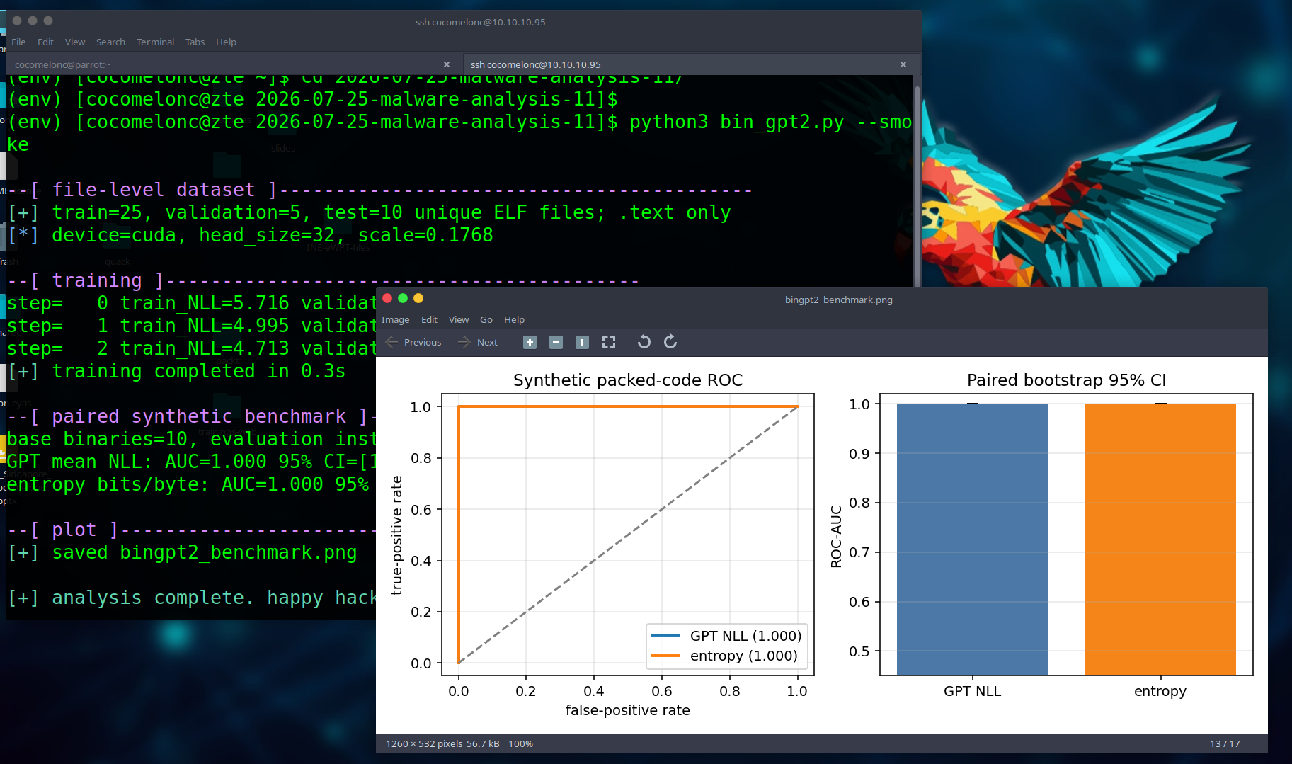
The ROC panel in bingpt2_benchmark.png compares both detectors. The second panel shows ROC-AUC with a paired bootstrap 95% confidence interval: resampling is performed by base binary, so an original file and its packed variant always stay together. FPR@95%TPR answers a more operational question than AUC alone: how many normal samples become false positives when the detector must catch 95% of packed samples.
There is no requirement for GPT to beat entropy here. LZMA compression creates an easy high-entropy distinction, so entropy may match or outperform the model. If that happens, the correct conclusion is that this synthetic benchmark does not demonstrate an advantage from learned byte order. The next research step is harder data: real benign packed executables, compressed resources as hard negatives, multiple compiler families, and confidence intervals over a larger file-level test set.
summary
| component | what it does |
|---|---|
GPT (60 lines) |
decoder-only transformer, 256-byte vocab, from scratch |
| training loop | next-byte prediction on normal code, ~25 s on a GPU |
generate() |
proves it learned x86 texture (readable opcodes) |
nll() / perplexity |
packing / anomaly detector, ROC-AUC 0.994 |
This is the whole point: a transformer is just a next-token predictor trained by gradient descent, and once you build one yourself it stops being a buzzword and becomes a tool. The exact same engine, scaled up, powers the LLM copilots appearing in SOCs today.
A few honest limitations. Perplexity flags unusual bytes, so legitimately compressed resources (icons, installers) will also look “surprising” - in production you combine this with PE/ELF section context and known-packer YARA rules. The model is also attackable: an adversary can pad a file with normal-looking code to lower average surprise. As always, one signal is never enough - use it as a fast lead, not a verdict.
In the next part we will go further and feed the model opcode sequences from a real disassembler (capstone) instead of raw bytes, which makes the “code grammar” even sharper for family classification.
I hope this post with practical examples is useful for malware researchers, reverse engineers and everyone interested in blue team and ML skills.
Malware analysis part 6: Shannon entropy
Malware analysis part 10: Practical PE parsing
Anti-DDoS: SYN flood detection
Attention Is All You Need (transformer paper)
Andrej Karpathy - nanoGPT
MalConv - malware detection from raw bytes
source code in github
This is a practical case for educational purposes only.
Thanks for your time happy hacking and good bye! PS. All drawings and screenshots are mine