Anti-DDoS research: detecting short traffic anomalies with Haar wavelets. Simple C example.

﷽

Hello, cybersecurity enthusiasts and white hackers!

Today I want to start a small defensive research series about DDoS detection mechanisms (Anti-DDoS). This research not used production architecture, no private telemetry, no vendor internals (since I sign my NDA with one of the best companies in my country). Just one simple idea, one small C program, and one reproducible graph.

The question for this post is:

Can a very small wavelet detector catch a short DDoS-like traffic pulse that a rolling average detector misses?

The short answer is yes. And the reason is mathematical: averaging hides short pulses, while Haar wavelet detail coefficients react to sharp changes.

idea

Many simple DDoS detectors start from a traffic rate:

packets per second
bytes per second
SYN/ACK ratio
DNS qps
UDP qps

A common first detector is a rolling average:

\[\bar{x}_t = \frac{1}{W}\sum_{i=0}^{W-1} x_{t-i}\]

Then we alert if:

\[\bar{x}_t > \theta\]

This is simple and useful, but it has one big problem: a short attack can be averaged away.

For example, if an attack sends a huge pulse only during a small part of the window, the rolling average sees only:

\[\bar{x}=pA\]

where:

\( A \) is attack amplitude;
\( p \) is pulse duty cycle.

If:

\[pA \le \theta\]

then the average detector does not alert.

But the network still suffers during the pulse. In real life this can mean packet drops, queue spikes, retransmissions, resolver overload, or increased p99 latency.

Haar wavelet

The simplest wavelet is the Haar wavelet. For two neighboring samples:

\[a_i = \frac{x_{2i} + x_{2i+1}}{\sqrt{2}}\] \[d_i = \frac{x_{2i+1} - x_{2i}}{\sqrt{2}}\]

The \(a_i\) value is an average-like component. The \(d_i\) value is a detail component.

In plain english:

average asks: “how high is traffic in the window?”
Haar detail asks: “how sharply did traffic change?”

For short DDoS pulses, the second question is often better.

If traffic jumps from 10k pps to 80k pps:

\[|d| = \frac{|80-10|}{\sqrt{2}} \approx 49.5\]

This is a strong signal even when the rolling average remains below threshold.

practical example

Let’s build a tiny C program. It does not send packets and does not attack anything. It only simulates traffic samples:

normal traffic is around 10k packets/sec;
two short DDoS-like pulses appear at t=120..122 and t=180..182;
rolling average uses a 16 sample window;
wavelet detector uses first-level Haar detail coefficients.

First of all, include headers:

#include <math.h>
#include <stdio.h>
#include <stdlib.h>
#include <string.h>

Define our sample size and baseline window:

#define N 256
#define AVG_WINDOW 16
#define BASELINE_N 100

The sample structure:

typedef struct {
  int t;
  double traffic;
  double rolling_avg;
  double haar_detail;
  double wavelet_score;
  int avg_alert;
  int wavelet_alert;
  int is_attack;
} sample_t;

Now we need robust statistics. I use median and MAD instead of mean and standard deviation. Why? Because attack spikes can poison mean and standard deviation.

\[\operatorname{MAD}(x)=\operatorname{median}(|x_i-\operatorname{median}(x)|)\]

Robust z-score:

\[z = \frac{x-\operatorname{median}(x)}{1.4826\cdot\operatorname{MAD}(x)}\]

The synthetic traffic function:

static double synthetic_traffic(int t) {
  double baseline = 10.0 + 1.5 * sin((2.0 * M_PI * t) / 64.0);
  double tiny_noise = (double)((t * 37) % 11) / 20.0;

  if (t >= 120 && t <= 122) {
    return 80.0 + tiny_noise;
  }
  if (t >= 180 && t <= 182) {
    return 70.0 + tiny_noise;
  }
  return baseline + tiny_noise;
}

As you can see, this is not a real pcap parser yet. This is intentional. First we prove the signal-processing idea in the cleanest possible setup. Then we can replace synthetic_traffic() with features extracted from pcap: packets/sec, bytes/sec, SYN rate, DNS qps, NXDOMAIN rate, and so on.

The Haar detail value is simple:

s[i].haar_detail = fabs(s[i].traffic - s[i - 1].traffic) / sqrt(2.0);

For the rolling average detector:

s[i].avg_alert = s[i].rolling_avg > avg_threshold;

For the wavelet detector:

s[i].wavelet_score = (s[i].haar_detail - med) / sigma;
s[i].wavelet_alert = s[i].wavelet_score > wavelet_threshold;

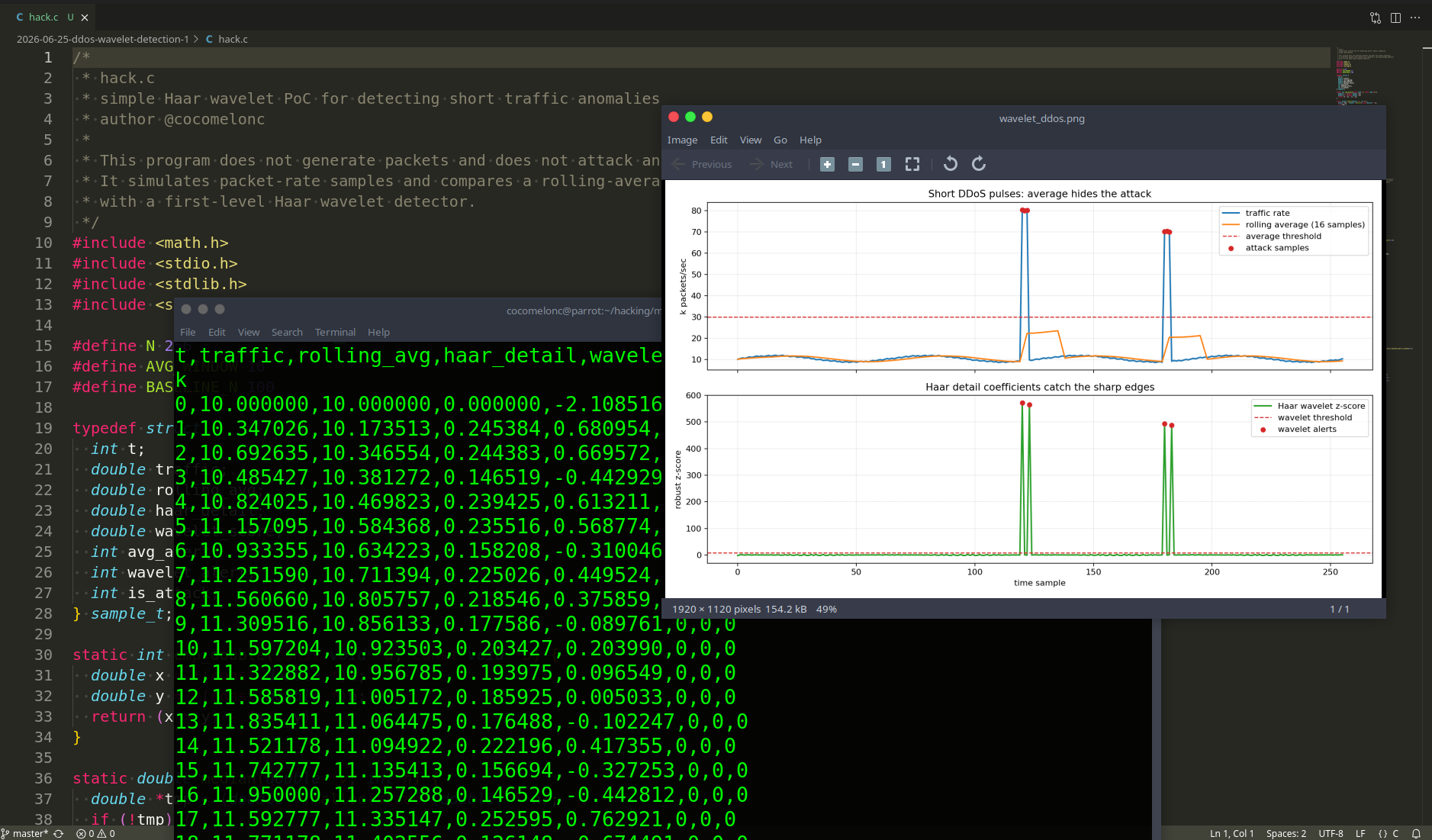
So the full source code of this example is looks like this (hack.c):

/*
 * hack.c
 * simple Haar wavelet PoC for detecting short traffic anomalies
 * author @cocomelonc
 *
 * This program does not generate packets and does not attack anything.
 * It simulates packet-rate samples and compares a rolling-average detector
 * with a first-level Haar wavelet detector.
 */
#include <math.h>
#include <stdio.h>
#include <stdlib.h>
#include <string.h>

#define N 256
#define AVG_WINDOW 16
#define BASELINE_N 100

typedef struct {
  int t;
  double traffic;
  double rolling_avg;
  double haar_detail;
  double wavelet_score;
  int avg_alert;
  int wavelet_alert;
  int is_attack;
} sample_t;

static int cmp_double(const void *a, const void *b) {
  double x = *(const double *)a;
  double y = *(const double *)b;
  return (x > y) - (x < y);
}

static double median(double *v, int n) {
  double *tmp = (double *)malloc(sizeof(double) * n);
  if (!tmp) {
    perror("malloc");
    exit(1);
  }

  memcpy(tmp, v, sizeof(double) * n);
  qsort(tmp, n, sizeof(double), cmp_double);

  double result;
  if (n % 2 == 0) {
    result = (tmp[n / 2 - 1] + tmp[n / 2]) / 2.0;
  } else {
    result = tmp[n / 2];
  }

  free(tmp);
  return result;
}

static double mad(double *v, int n, double med) {
  double *dev = (double *)malloc(sizeof(double) * n);
  if (!dev) {
    perror("malloc");
    exit(1);
  }

  for (int i = 0; i < n; i++) {
    dev[i] = fabs(v[i] - med);
  }

  double result = median(dev, n);
  free(dev);

  if (result < 1e-9) {
    return 1e-9;
  }
  return result;
}

static int is_attack_time(int t) {
  return (t >= 120 && t <= 122) || (t >= 180 && t <= 182);
}

static int in_event_window(int t, int start, int end) {
  return t >= start && t <= end + 1;
}

static double synthetic_traffic(int t) {
  double baseline = 10.0 + 1.5 * sin((2.0 * M_PI * t) / 64.0);
  double tiny_noise = (double)((t * 37) % 11) / 20.0;

  if (t >= 120 && t <= 122) {
    return 80.0 + tiny_noise;
  }
  if (t >= 180 && t <= 182) {
    return 70.0 + tiny_noise;
  }
  return baseline + tiny_noise;
}

int main(void) {
  sample_t s[N];
  double baseline_details[BASELINE_N - 1];

  for (int i = 0; i < N; i++) {
    s[i].t = i;
    s[i].traffic = synthetic_traffic(i);
    s[i].is_attack = is_attack_time(i);

    int start = i - AVG_WINDOW + 1;
    if (start < 0) {
      start = 0;
    }

    double sum = 0.0;
    int count = 0;
    for (int j = start; j <= i; j++) {
      sum += s[j].traffic;
      count++;
    }

    s[i].rolling_avg = sum / (double)count;
    s[i].haar_detail = 0.0;
    if (i > 0) {
      s[i].haar_detail = fabs(s[i].traffic - s[i - 1].traffic) / sqrt(2.0);
    }
  }

  for (int i = 1; i < BASELINE_N; i++) {
    baseline_details[i - 1] = s[i].haar_detail;
  }

  double med = median(baseline_details, BASELINE_N - 1);
  double sigma = 1.4826 * mad(baseline_details, BASELINE_N - 1, med);

  const double avg_threshold = 30.0;
  const double wavelet_threshold = 8.0;

  for (int i = 0; i < N; i++) {
    s[i].wavelet_score = (s[i].haar_detail - med) / sigma;
    s[i].avg_alert = s[i].rolling_avg > avg_threshold;
    s[i].wavelet_alert = s[i].wavelet_score > wavelet_threshold;
  }

  int event_start[] = {120, 180};
  int event_end[] = {122, 182};
  int event_count = 2;

  int avg_event_tp = 0;
  int wav_event_tp = 0;

  for (int e = 0; e < event_count; e++) {
    int avg_seen = 0;
    int wav_seen = 0;
    for (int i = 0; i < N; i++) {
      if (!in_event_window(i, event_start[e], event_end[e])) {
        continue;
      }
      if (s[i].avg_alert) {
        avg_seen = 1;
      }
      if (s[i].wavelet_alert) {
        wav_seen = 1;
      }
    }
    avg_event_tp += avg_seen;
    wav_event_tp += wav_seen;
  }

  int avg_event_fp = 0;
  int wav_event_fp = 0;
  for (int i = 0; i < N; i++) {
    int inside_any_event = 0;
    for (int e = 0; e < event_count; e++) {
      if (in_event_window(i, event_start[e], event_end[e])) {
        inside_any_event = 1;
      }
    }
    if (!inside_any_event && s[i].avg_alert) {
      avg_event_fp++;
    }
    if (!inside_any_event && s[i].wavelet_alert) {
      wav_event_fp++;
    }
  }

  int avg_event_fn = event_count - avg_event_tp;
  int wav_event_fn = event_count - wav_event_tp;

  FILE *f = fopen("wavelet_ddos.csv", "w");
  if (!f) {
    perror("fopen");
    return 1;
  }

  fprintf(f, "t,traffic,rolling_avg,haar_detail,wavelet_score,avg_alert,wavelet_alert,is_attack\n");
  for (int i = 0; i < N; i++) {
    fprintf(f, "%d,%.6f,%.6f,%.6f,%.6f,%d,%d,%d\n",
      s[i].t,
      s[i].traffic,
      s[i].rolling_avg,
      s[i].haar_detail,
      s[i].wavelet_score,
      s[i].avg_alert,
      s[i].wavelet_alert,
      s[i].is_attack);
  }
  fclose(f);

  printf("baseline Haar detail median: %.6f\n", med);
  printf("baseline Haar detail robust sigma: %.6f\n", sigma);
  printf("rolling average threshold: %.2f\n", avg_threshold);
  printf("wavelet z-score threshold: %.2f\n\n", wavelet_threshold);

  printf("event-level rolling average detector: TP=%d FP=%d FN=%d\n",
    avg_event_tp, avg_event_fp, avg_event_fn);
  printf("event-level Haar wavelet detector:    TP=%d FP=%d FN=%d\n",
    wav_event_tp, wav_event_fp, wav_event_fn);
  printf("\nwrote wavelet_ddos.csv\n");

  return 0;
}

demo

Compile it:

gcc -O2 -Wall -Wextra hack.c -lm -o hack

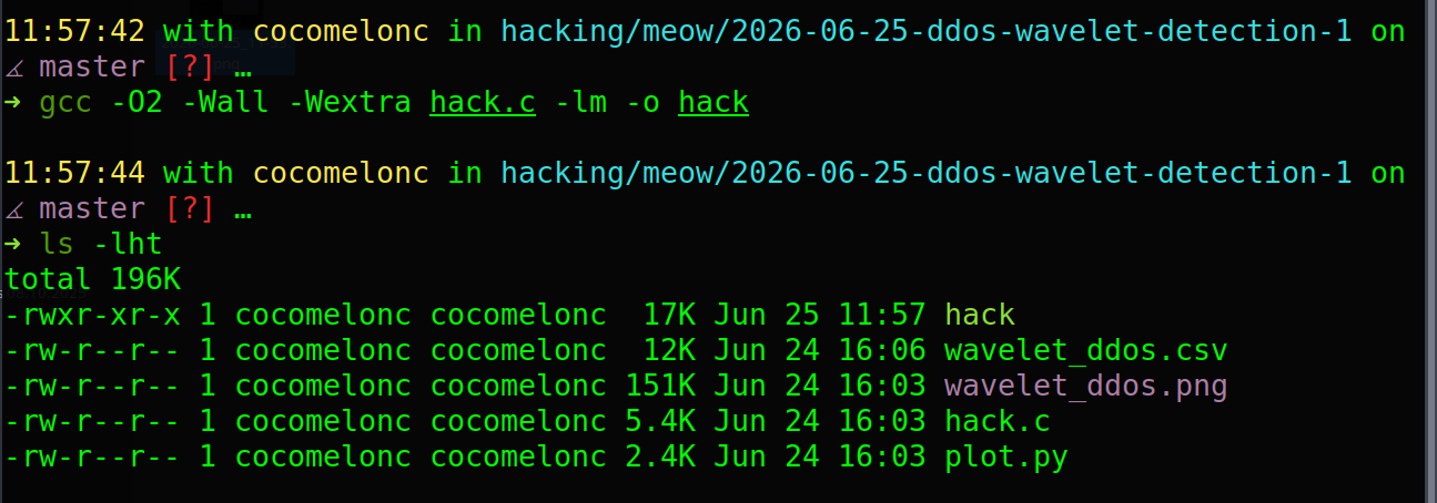
Run:

./hack

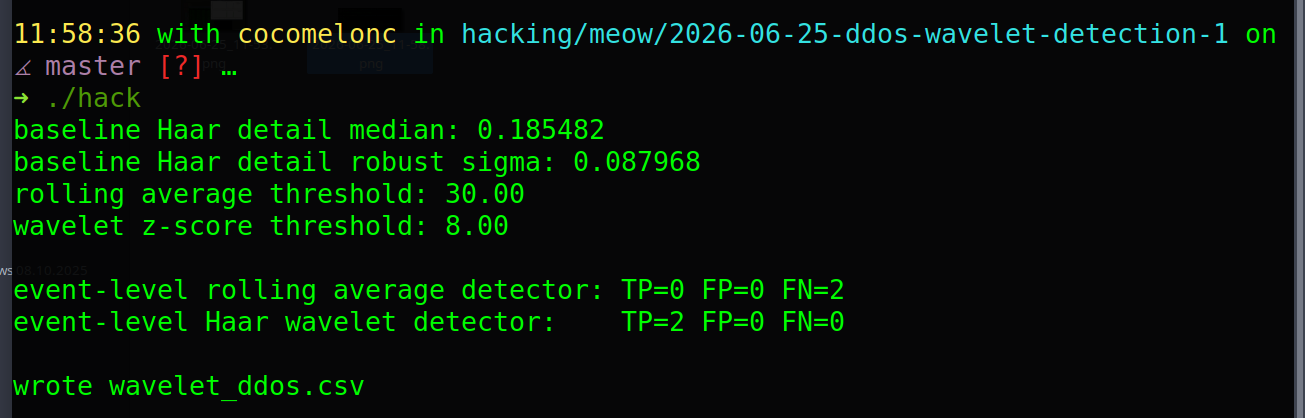
As you can see, in my case:

baseline Haar detail median: 0.185482
baseline Haar detail robust sigma: 0.087968
rolling average threshold: 30.00
wavelet z-score threshold: 8.00

event-level rolling average detector: TP=0 FP=0 FN=2
event-level Haar wavelet detector:    TP=2 FP=0 FN=0

wrote wavelet_ddos.csv

This is the important line:

event-level rolling average detector: TP=0 FP=0 FN=2
event-level Haar wavelet detector:    TP=2 FP=0 FN=0

The rolling average misses both short events. The Haar wavelet detector catches both.

drawing the graph

For the article I used this small Python script only for plotting the CSV generated by the C program:

#!/usr/bin/env python3
import csv

import matplotlib.pyplot as plt


def read_csv(path):
    rows = []
    with open(path, newline="") as f:
        for row in csv.DictReader(f):
            rows.append({
                "t": int(row["t"]),
                "traffic": float(row["traffic"]),
                "rolling_avg": float(row["rolling_avg"]),
                "haar_detail": float(row["haar_detail"]),
                "wavelet_score": float(row["wavelet_score"]),
                "avg_alert": int(row["avg_alert"]),
                "wavelet_alert": int(row["wavelet_alert"]),
                "is_attack": int(row["is_attack"]),
            })
    return rows


def main():
    rows = read_csv("wavelet_ddos.csv")

    t = [r["t"] for r in rows]
    traffic = [r["traffic"] for r in rows]
    rolling = [r["rolling_avg"] for r in rows]
    score = [r["wavelet_score"] for r in rows]
    attack_t = [r["t"] for r in rows if r["is_attack"]]
    attack_y = [r["traffic"] for r in rows if r["is_attack"]]
    wav_alert_t = [r["t"] for r in rows if r["wavelet_alert"]]
    wav_alert_y = [r["wavelet_score"] for r in rows if r["wavelet_alert"]]

    fig, axes = plt.subplots(2, 1, figsize=(12, 7), sharex=True)

    axes[0].plot(t, traffic, label="traffic rate", color="#1f77b4", linewidth=1.8)
    axes[0].plot(t, rolling, label="rolling average (16 samples)", color="#ff7f0e", linewidth=1.6)
    axes[0].axhline(30.0, color="#d62728", linestyle="--", linewidth=1.2, label="average threshold")
    axes[0].scatter(attack_t, attack_y, color="#d62728", s=28, label="attack samples", zorder=5)
    axes[0].set_ylabel("k packets/sec")
    axes[0].set_title("Short DDoS pulses: average hides the attack")
    axes[0].grid(True, alpha=0.25)
    axes[0].legend(loc="upper right")

    axes[1].plot(t, score, label="Haar wavelet z-score", color="#2ca02c", linewidth=1.8)
    axes[1].axhline(8.0, color="#d62728", linestyle="--", linewidth=1.2, label="wavelet threshold")
    axes[1].scatter(wav_alert_t, wav_alert_y, color="#d62728", s=28, label="wavelet alerts", zorder=5)
    axes[1].set_xlabel("time sample")
    axes[1].set_ylabel("robust z-score")
    axes[1].set_title("Haar detail coefficients catch the sharp edges")
    axes[1].grid(True, alpha=0.25)
    axes[1].legend(loc="upper right")

    fig.tight_layout()
    fig.savefig("wavelet_ddos.png", dpi=160)
    print("wrote wavelet_ddos.png")


if __name__ == "__main__":
    main()

Run:

python3 plot.py

As a result:

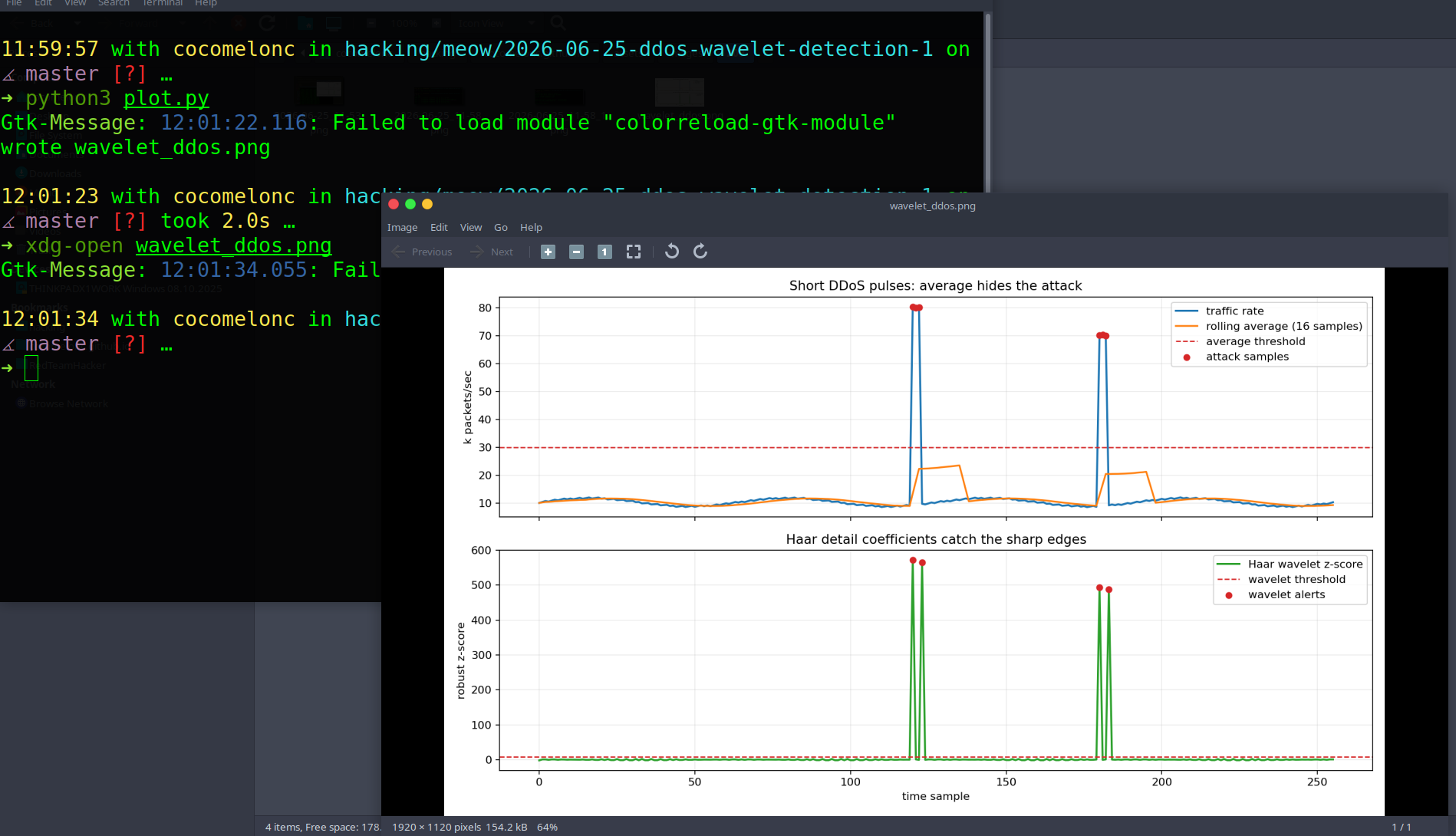
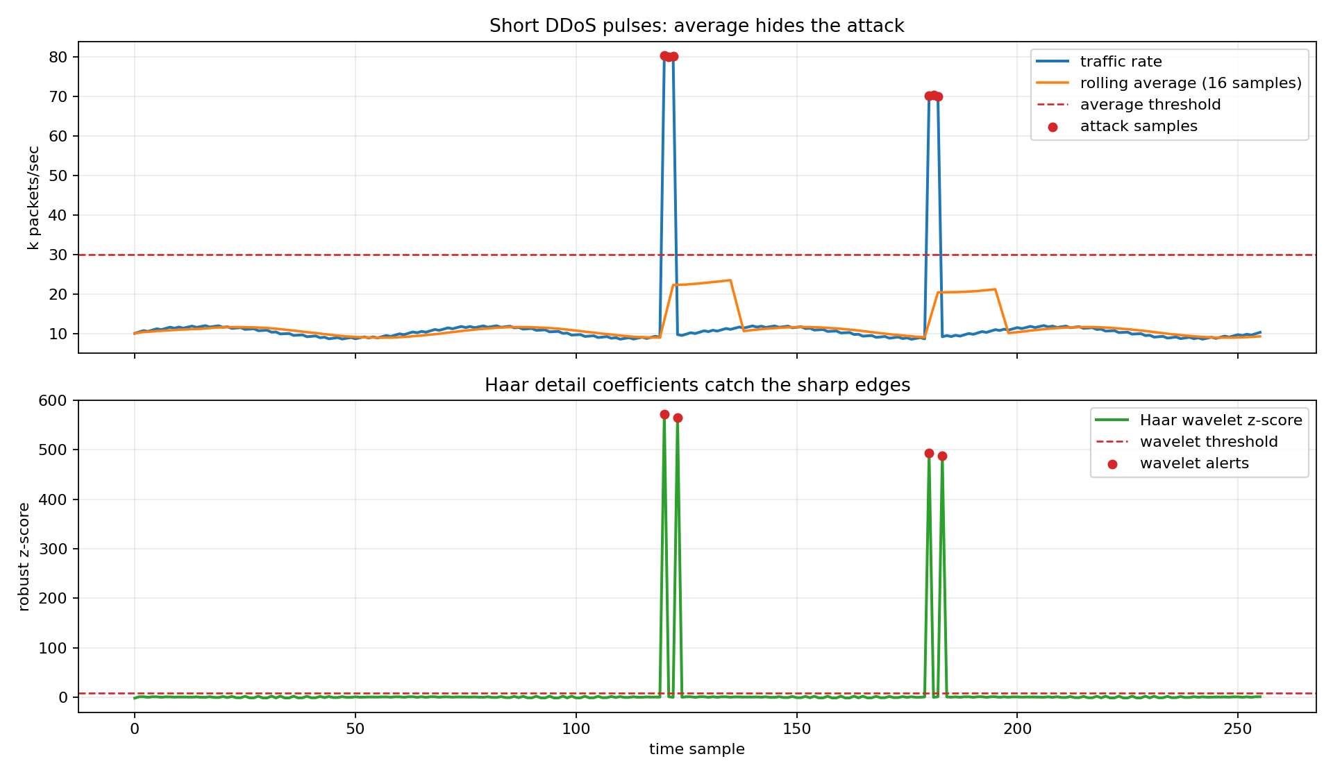
The upper plot shows the main trick. The raw traffic has short spikes, but the rolling average does not cross the threshold. The lower plot shows the Haar wavelet score. It immediately spikes on the rising and falling edges.

why this works???

The average detector is a low-pass filter. It smooths the signal. This is useful for removing noise, but bad for short attacks.

If a pulse has amplitude (A) and duty cycle (p), the average sees:

\[pA\]

The detector misses when:

\[pA \le \theta\]

But Haar detail sees the jump:

\[|d| = \frac{|x_t-x_{t-1}|}{\sqrt{2}}\]

For a jump from normal traffic (B) to attack traffic (A):

\[|d| = \frac{|A-B|}{\sqrt{2}}\]

This does not shrink with the duty cycle in the same way the average does. That is why wavelets are useful for short DDoS pulses, microbursts, and low-rate on/off attacks.

cybersecurity interpretation

This is not a complete Anti-DDoS system. It is one detector feature.

In a real system I would not alert only on one wavelet spike. I would combine it with protocol features:

UDP flood: packets/sec, bytes/sec, source port distribution, packet size buckets.
SYN flood: SYN/SYN-ACK/ACK ratios, incomplete handshakes.
DNS flood: qps, unique qnames, NXDOMAIN ratio, qtype distribution.
Fragmentation attack: fragment rate, incomplete reassembly ratio, tiny fragments.

The wavelet detector answers a specific question:

Did traffic change too sharply compared with the normal baseline?

That question is valuable because many operational problems happen during short bursts before long-window metrics become alarming.

where to get real pcaps

For the next steps, public datasets are better than private production traffic:

CICDDoS2019 from Canadian Institute for Cybersecurity - this dataset includes benign traffic, DDoS attacks, raw PCAPs, and flow CSV files. It includes attacks such as DNS, LDAP, MSSQL, NetBIOS, NTP, SNMP, SSDP, UDP, UDP-Lag, SYN, TFTP, and WebDDoS.

CAIDA DDoS Attack 2007 - this is about one hour of anonymized DDoS attack traffic split into 5-minute pcap files. It requires CAIDA access approval and has an acceptable-use agreement.

MAWI traffic archive - this is useful for background traffic and anomaly research. It is not as convenient as a labeled DDoS dataset, but it is good for studying real backbone traffic behavior.

UNSW-NB15 - this is a broader intrusion detection dataset. It is useful for feature extraction experiments, but for a focused DDoS article I would start with CICDDoS2019 or CAIDA.

what to do next

This post proves only one small thing:

A first-level Haar wavelet detector can catch short pulse anomalies that a rolling average detector misses.

The next practical steps:

replace synthetic traffic with packet-rate extracted from a public pcap.
compare rolling average vs Haar wavelet on CICDDoS2019 UDP or SYN attack windows.

add entropy:

\[H(X)=-\sum_i p_i\log p_i\]

add a combined score:

\[S = w_1Z_{rate}+w_2Z_{wavelet}+w_3Z_{entropy}\]

measure detection delay, false positives, and false negatives.

conclusion

The point of this post is not that Haar wavelets are magic. They are not. The point is that DDoS detection should look at the shape of traffic, not only its average.

For short traffic pulses:

• rolling average can miss the attack;
• Haar wavelet detail coefficients expose the sharp change;
• robust z-score gives a simple thresholding method;
• the whole idea can be implemented in a few lines of C.

This is a good first building block for a deeper Anti-DDoS research series.

references and further reading

If you want to go deeper into the math and the research behind this post, here are the academic papers I recommend. I grouped them by topic.

Wavelets and signal analysis of network traffic

P. Barford, J. Kline, D. Plonka, A. Ron. A Signal Analysis of Network Traffic Anomalies (ACM SIGCOMM Internet Measurement Workshop, 2002) - pdf. The classic paper on using wavelet decomposition to expose short-lived traffic anomalies.
S. Mallat. A Theory for Multiresolution Signal Decomposition: The Wavelet Representation (IEEE Trans. PAMI, 1989) - doi. The foundational multiresolution analysis paper behind the Haar/DWT machinery.
I. Daubechies. Ten Lectures on Wavelets (SIAM, 1992) - doi. The standard reference textbook for wavelet theory.
C.-M. Cheng, H. T. Kung, K.-S. Tan. Use of Spectral Analysis in Defense Against DoS Attacks (IEEE GLOBECOM, 2002) - pdf. Spectral/power-density view of DoS traffic, a close cousin of the wavelet approach.

Low-rate and pulsing DDoS attacks

A. Kuzmanovic, E. W. Knightly. Low-Rate TCP-Targeted Denial of Service Attacks (The Shrew vs. the Mice and Elephants) (ACM SIGCOMM, 2003) - pdf. Explains exactly why low duty-cycle pulses evade average-based detectors while still hurting TCP.

Change-point detection (onset detection)

E. S. Page. Continuous Inspection Schemes (Biometrika, 1954) - doi. The original CUSUM change-detection scheme.
G. V. Moustakides. Optimal Stopping Times for Detecting Changes in Distributions (Annals of Statistics, 1986) - doi. Proves the minimax optimality of CUSUM for minimum-delay detection.
H. Wang, D. Zhang, K. G. Shin. Detecting SYN Flooding Attacks (IEEE INFOCOM, 2002) - pdf. Non-parametric CUSUM applied to the SYN-FIN difference; directly relevant to SYN-flood detection.

Entropy and statistical / distributional detection

L. Feinstein, D. Schnackenberg, R. Balupari, D. Kindred. Statistical Approaches to DDoS Attack Detection and Response (DARPA DISCEX, 2003) - doi. Entropy and chi-square tests for volume-independent detection.
A. Lall, V. Sekar, M. Ogihara, J. Xu, H. Zhang. Data Streaming Algorithms for Estimating Entropy of Network Traffic (ACM SIGMETRICS, 2006) - pdf. How to estimate traffic entropy at line rate with small memory.
A. Lakhina, M. Crovella, C. Diot. Diagnosing Network-Wide Traffic Anomalies (ACM SIGCOMM, 2004) - pdf. PCA subspace method for correlated, network-wide anomalies.

Robust statistics (median / MAD / z-score)

P. J. Huber. Robust Estimation of a Location Parameter (Annals of Mathematical Statistics, 1964) - doi. The origin of robust location estimation behind median/MAD.
F. R. Hampel. The Influence Curve and Its Role in Robust Estimation (JASA, 1974) - doi. Breakdown point and influence functions, why MAD beats standard deviation under contamination.

Baseline modeling and seasonality

J. D. Brutlag. Aberrant Behavior Detection in Time Series for Network Monitoring (USENIX LISA, 2000) - pdf. Holt-Winters seasonal baselining with confidence bands - the operational version of an adaptive threshold.

Self-similar traffic (background for why wavelets fit network data)

W. E. Leland, M. S. Taqqu, W. Willinger, D. V. Wilson. On the Self-Similar Nature of Ethernet Traffic (ACM SIGCOMM, 1993) - doi. Shows network traffic is self-similar/bursty across scales, which motivates multi-resolution analysis.

Surveys and datasets

J. Mirkovic, P. Reiher. A Taxonomy of DDoS Attack and DDoS Defense Mechanisms (ACM SIGCOMM CCR, 2004) - doi. A good map of the whole attack/defense landscape.
I. Sharafaldin, A. H. Lashkari, S. Hakak, A. A. Ghorbani. Developing Realistic Distributed Denial of Service (DDoS) Attack Dataset and Taxonomy (IEEE ICCST, 2019) - doi. The paper behind the CICDDoS2019 dataset linked above.

source code in github

This is a practical defensive case for educational purposes only.

Thanks for your time happy hacking and good bye! PS. All drawings and screenshots are mine