Malware analysis - part 1: My intro to x86 assembly.

﷽

Hello, cybersecurity enthusiasts and white hackers!

malware analysis

Any person who considers himself close to the world of information security, especially malware analysts (blue team) and exploit developers (red team), must have a basic understanding of assembly language.

As I wrote earlier in my posts, I came to cybersecurity with programming experience, but I only have experience in red team scenarios, so I want to try up my skills in blue team, especially in malware analysis.

Today, malware analysis is a whole industry in the field of information security. Antivirus engines laboratories that release their own protection products, highly specialized groups of experts striving to be in the trend of attack vectors, and even malware writers themselves, who compete for a potential client - “victim”, are also involved in it.

So I will start a series of articles dedicated to my path in learning this craft.

I really hope that this will help at least one person other than me.

Let’s go!

In traditional computer architecture, a computer system can be represented as several levels of abstraction that create a way of hiding the implementation details.

For simplicity, we will assume that we have three levels of coding when analyzing malware.

This is very simplest model, in real life computer systems are generally described with more than three levels of abstraction:

HARDWARE - the hardware level, the only physical level, consists of electrical circuits that implement complex combinations of logical operators such as XOR, AND, OR, and NOT gates, known as digital logic. Because of its physical nature, hardware cannot be easily manipulated by software.

MICROCODE - also known as firmware. Microcode operates only on the exact circuitry for which it was designed. It contains microinstructions that translate from the higher machine-code level to provide a way to interface with the hardware.

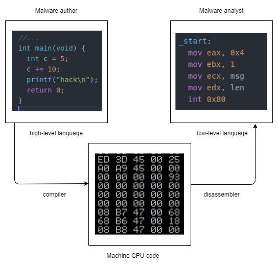
MACHINE CODE - the machine code level consists of opcodes, hexadecimal digits that tell the processor what you want it to do. It’s not just one language called machine code. It’s many different kinds of machine code. Just as we speak different languages as people, machines speak different languages.

LOW-LEVEL LANGUAGES - a low-level languages is a human-readable version of a computer architecture’s instruction set. The most common low-level language is assembly language. Assembly language which corresponds to the different architectures is by far the most important tool in any malware analyst’s toolkit.

HIGH-LEVEL LANGUAGES - Most computer programmers include who write malware, operate at the level of high-level languages. High-level languages provide strong abstraction from the machine level and make it easy to use programming logic and flow-control mechanisms.

INTERPRETED LANGUAGES - Interpreted languages are at the top level. The code at this level is not compiled into machine code, instead, it is translated into bytecode. Bytecode executes within an interpreter, which is a program that translates bytecode into executable machine code on the fly at runtime. For example, python. Python is well suited for quick malware analysis. For example, a library such as pefile. In one of the following posts I will show an example of using this library.

The term “reverse engineering” has several popular meanings. In my case, I am considering researching compiled programs (malware). When we disassemble malware, we take the malware bin as input then we generate assembly language code as output, usually with a disassembler.

I think many more experienced malware analysts will agree with me if I start with a short introduction to assembly language x86.

the x86 architecture

At this time there two main architectures that indicate how our programs is compiled and executed: 32-bit and 64-bit. We will be going over the 32-bit architecture (x86) and 32-bit (x86) assembly language.

The internals of most modern computers architectures, including x86, follow the Von Neumann architecture:
CPU (Central Processing Unit) - executes code.
RAM - the main memory of the system stores all data and node.
I/O - an input/output system interfaces with devices such as hard drives, keyboards, printers etc.

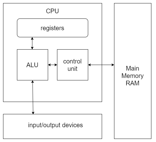
As you can see CPU contains several components:
The control unit gets instructions to execute from RAM using a register - the instruction pointer, which stores the address of the instruction to execute.

Registers - Registers are small memory storage areas built into the processor (still volatile memory).
There are 8 “general purpose” registers:
EAX - stores function return values
EBX - base pointer to the data section
ECX - counter for string and loop operations
EDX - I/O pointer
ESI - source pointer for string operations
EDI - destination pointer for string operations
ESP - stack pointer
EBP - stack frame base pointer

And instruction pointer:
EIP - pointer to next instruction to execute - “instruction pointer”

The ALU - Arithmetic logic unit executes an instruction fetched from RAM and places the results in registers or memory. The process of fetching and executing instruction after instruction is repeated as a program runs.

The main memory RAM for a single program can be divided into the following 4 main sections:

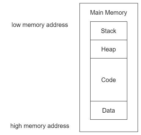
The Data section contains values that are put in place when a program is initially loaded.
Code includes the instructions fetched by the CPU to execute the program’s tasks.
Heap is used for dynamic memory during program execution, to allocate new values (for example malloc() and calloc() functions in C) and eliminate (for example free() function in C) values that the program no longer needs.
The Stack is used for local variables and parameters for functions and to help control program flow.

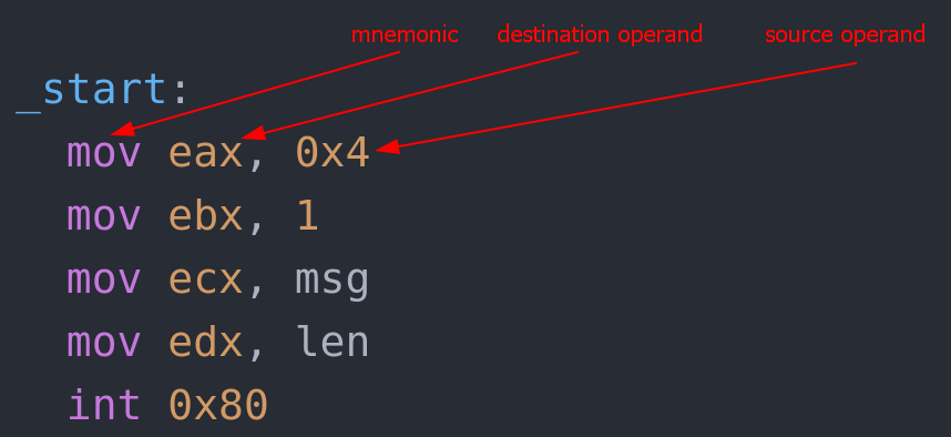
instructions

Instructions are building blocks of assembly programs. In x86 assembly, an instruction is made of a mnemotic and 0 or more operands:

The EFLAGS register holds many single bit flags.
For now, we remember the following flags:
ZF - Zero Flag - Set if the result of some instruction is zero; cleared otherwise
SF - Sign Flag - Set equal to the most-significant bit of the result, which is the sign bit of a signed integer: 0 - indicates positive value, 1 - indicates a negative value

NOP nop - first x86 instuction, no operation! no registers! no values! This instruction just for paddding bytes or delay time.
Red teamers use it to make simple exploits more reliable.

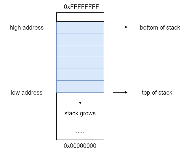
Before looking at other instructions, we need to elaborate on the concept of a stack in memory.

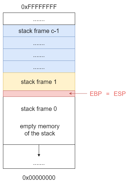
The Stack is conceptual are of main memory (RAM) which is designated by the operating system when program is started. A stack is a LIFO (Last-In-First-Out) data structure where data is “pushed” on to the top of the stack and “popped” off the top. By convention the stack grows toward lower memory addresses:

The Stack is logically divided into many Stack Frames.

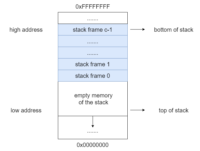
The newest stack frame is indexed as Stack Frame 0, the older one Stack Frame 1, and the oldest Stack Frame is indexed Stack Frame (count - 1)

The current stack frame (Stack Frame 0) is always the newest Stack Frame.

A stack frame is represented by two pointers:
Base pointer saved in EBP register - the memory address that is equal to (EBP-1) is the first memory location of the stack frame.
Stack pointer saved in ESP register - the memory address that is equal to (ESP) is the top memory location of the stack frame.

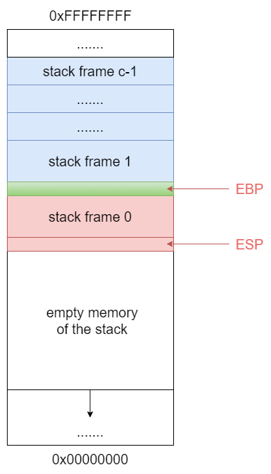
When Pushing or Popping values, ESP register value is changed (the stack pointer moves)
Base pointer value in EBP never change unless the current Stack Frame is changed.
The Stack Frame is empty when EBP value = ESP value.

All the space between these two registers make up the Stack Frame of whatever function is currently being called.

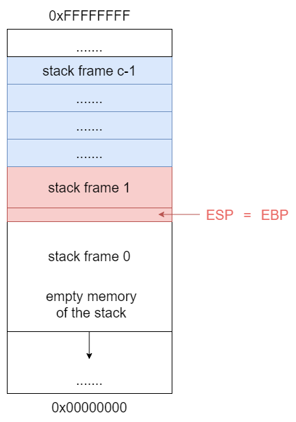
So, whenever a function is called a new Stack Frame is created. Local variables are also allocated at the bottom of the created Stack Frame. To create a new Stack Frame, simply change EBP value to be equal to ESP:

Now EBP = ESP, this means that the newest Stack Frame is empty. The previous stack frame now is indexed as Stack Frame 1.

But there are the caveat. This time we should save EBP value before changing it!.
First, PUSH value of EBP to save it:

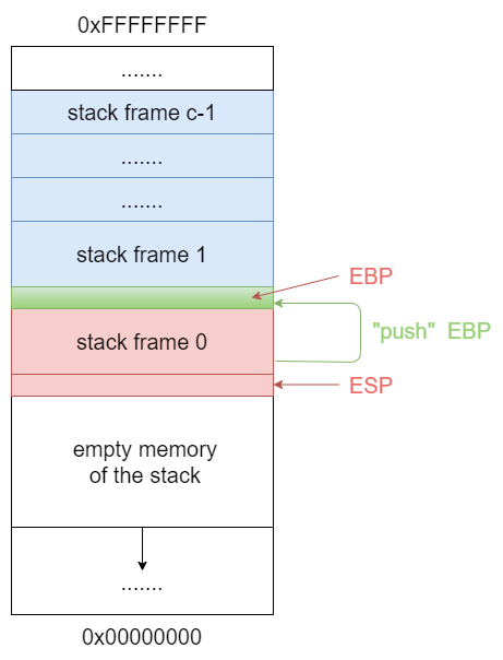
Then change the value of EBP:

All the stack addresses outside of the current stack frame are considered to be junked by the compiler.

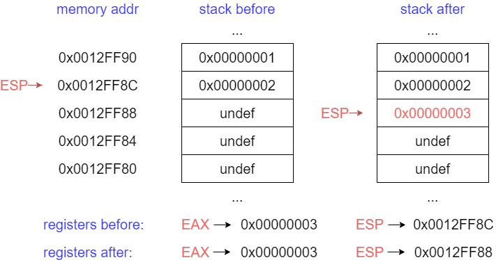
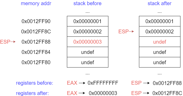
PUSH - push word, dword, qword onto the Stack.
For our purposes, it will always be a DWORD (4 bytes). Can either be an immediate (a numberic constant), or the value in a register. The push instruction automatically decrements the stack pointer ESP by 4.
For example:

push eax, 0x00000003

POP - pop a value from the Stack.
Take a DWORD off the stack, put it in a register, and increment ESP by 4.
For example:

pop eax

Before proceeding with other instructions let’s focus on call types (or calling convensions).

Calling conventions are a standardized method for functions to be implemented and called by the machine. A calling convention specifies the method that a compiler sets up to access a subroutine.

Calling conventions specify how arguments are passed to a function, how return values are passed back out of a function, how the function is called, and how the function manages the stack and its stack frame. In short, the calling convention specifies how a function call in C or C++ is converted into assembly language.

There are many call types, two of them are commmonly used in most programming languages:
cdecl - the default call type for C functions. The caller is responsible of cleaning the stack frame.
stdcall - the default call type for Win32 APIs. The callee is responsible of cleaning the stack frame.

CALL - call procedure.
This instruction job is to transfer control to a different function, in way that control can later be resumed where it left off. First it pushes the address of the next instruction onto the stack. Then it changes EIP to the address given in the instruction. Destination address can be specified in multiple ways:

• Absolute address
• Relative address (relative to the end of the instuction)

RET - return from procedure.
There are two forms of this instruction:

• Pop of the top of the stack into EIP, just written:

    ret
  

Typically used by cdecl functions.

• Pop of the top of the stack into EIP and add a constant number of bytes to ESP:

    ret 0x8
    ;....
    ;....
    ret 0x20
  

Typically used by stdcall functions.

MOV - can move:

1. register to register
2. memory to register, register to memory
3. immediate to register, immediate to memory
4. Never! memory to memory

Examples:

mov eax, ebx           ; copies the contents of EBX to the EAX register
mov eax, 0x42          ; copies the value 0x42 into EAX register

first x86 assembly language program

I appreciate everyone for your patience, if you have read this far. So finally we can try to code our first program in assmebly language. As I said earlier, we are going to create 32-bit assembly programs as most malware is written in 32-bit mode, but keep in mind: most of us all have 64-bit operating systems nowadays, 32-bit programs can run on them.

Let’s go!
I will write our programs for linux, I choose Ubuntu 16.04 64-bit.
First of all, please install NASM:

sudo apt-get install nasm

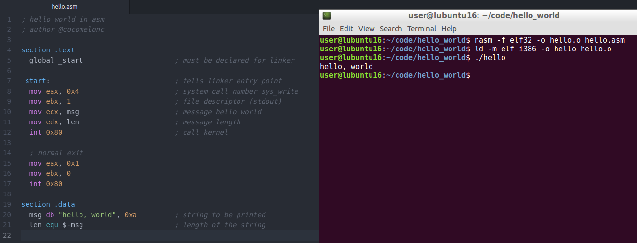
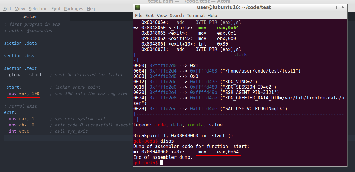
Then create test1.asm with following code:

; first program in asm
; author @cocomelonc

section .data

section .bss

section .text
  global _start   ; must be declared for linker

_start:           ; linker entry point
  mov eax, 100    ; mov 100 into the EAX register

; normal exit
exit:
  mov eax, 1      ; sys_exit system call
  mov ebx, 0      ; exit code 0 successfull execution
  int 0x80        ; call sys_exit

Every assembly language program is divided into three sections:
data section - this section is used for declaring initialized data or constants as this data does not ever change at runtime. You can declare constant values, buffer sizes, file names, etc.
bss section - this section is used for declaring uninitialized data or variables.
text section - this section is used for the actual code sections as it begins with a global _start which tells the kernel where execution begins.

Let’s go to compile our program:

nasm -f elf32 -o test1.o test1.asm
ld -m elf_i386 -o test1 test1.o

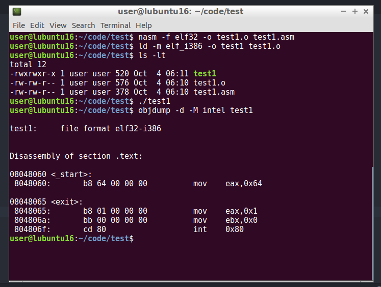
As you can see when we run it by ./test1 nothing happen. There is no output, and that’s correct. Because, all we did was create a program which move 100 to EAX register and normally exit.
And as you can see from output of command:

objdump -d -M intel test1

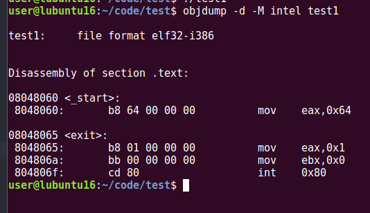
Since we consider the study from the point of view of a malware analyst, objdump command is very important and must have knowledge for static analysis.

Static analysis is the process of analyzing malware “at rest”, to extract identifying features and other characteristics from the tool without actually executing it.

The objdump utility is part of the binutils package, which is a bundle of tools used in Linux/UNIX systems for working with many core binary file types. The objdump utility is designed to be a full metadata analysis and reporting tool for executable files. Using the -d arguments, objdump can be told to disassemble the file.

Let’s back to our code and examine 15-18 lines.

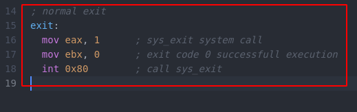
On line 16, in the Intel syntax we mov eax, 1 meaning we move the decimal value of 1 into eax which specifies the sys_exit call which will properly terminate program execution back to Linux so that there is no segmentation fault. (1)
Then on line 17 we mov ebx, 0 which moves 0 into ebx to show that the program successfully executed. (2)

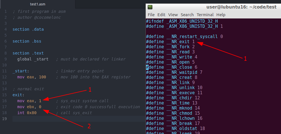
All the syscalls are listed in /usr/include/asm/unistd_32.h, together with their numbers (the value to put in EAX before you call int 0x80).

And finally, on line 18 we see int 0x80. Let’s dive into this a little deeper.

In Linux, there are two distinct areas of memory. At the very bottom of memory in any program execution we have the Kernel Space which is made up of the Dispatcher section and the Vector Table.
At the very top of memory in any program execution we have the User Space which is made up of The Stack, The Heap and finally your code all of which can be illustrated in the below diagram:

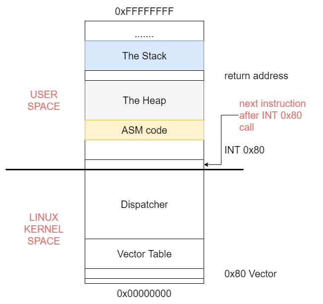
When we load the values as we demonstrated above and call INT 0x80, the very next instruction’s address in the User Space, ASM Code section which is your code, is placed into the Return Address area in The Stack. This is critical so that when INT 0x80 does its work, it can properly know what instruction is to be carried out next to ensure proper and sequential program execution.

Keep in mind in modern versions of Linux, we are utilizing Protected Mode which means you do NOT have access to the Linux Kernel Space. Everything under the long line that runs in the middle of the diagram above represents the Linux Kernel Space.

The natural question is why can’t we access this? The answer is very simple, Linux will NOT allow your code to access operating system internals as that would be very dangerous as any Malware could manipulate those components of the OS to track all sorts of things such as user keystrokes, activities and the like.

In addition, modern Linux OS architecture changes the address of these key components constantly as new software is installed and removed in addition to system patches and upgrades. This is the cornerstone of Protected Mode operating systems.

Firstly, I will not necessarly look at malware as I would rather focus on the topics of assembly language programs that will give you the tools and undestanding, and I want to first learn to understand at least a little bit of any program in assembler, not only malware.

I will continue the basic statistical analysis of our file, in order to understand what other tools may be useful for malware analysis.

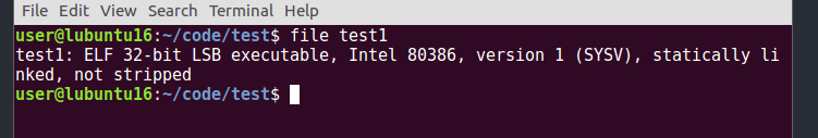
The file command is built in to pretty much every Linux and BSD. It is build around libmagic which is a library that can perform metadata analysis based upon arbitrary file structure information stored in a “magic database”:

file test1

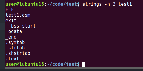
The strings tool is also part of the binutils package. This utility scans the file from beginning to end and attempts to discover strings that would be encoded using standard conventions, such as a sequence of human-readable characters followed by the \0 (NULL) byte (\x00). The strings utility can be told to change its behavior to filter only to longer-sized strings, and also can identify a number of different string encodings, such as the UTF-16 that is popular on Windows.
To show only 3-byte or greater strings:

strings -n 3 test1

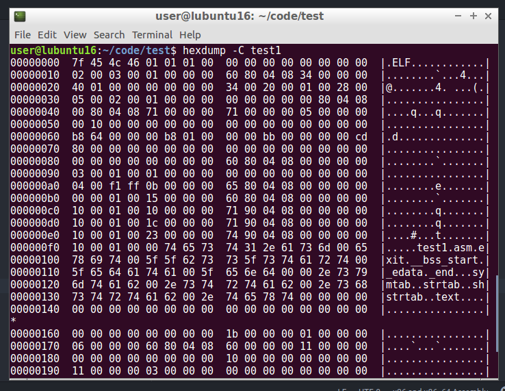
And my favourite one is hexdump. The hexdump command in Linux is used to filter and display the specified files, or standard input in a human readable specified format. My favorite invocation of hexdump is using the -C option. This gives a 16-byte-wide hexadecimal dump output, as well as a preview of the raw text (sanitizing unprinable characters) on the right. This gives you the ability to see the numeric representation, as well as view the raw data for human-readable content or other patterns that are helped by a denser viewport.

hexdump -C test1

The next thing I want to do is let’s take my test1 to GDB debugger tool, and examine what exactly is going on at the assembly level.

Before we start working with gdb, we need to install the gdb peda extension.

Let’s begin by loading my binary to gdb.

Run:

gdb -q test1

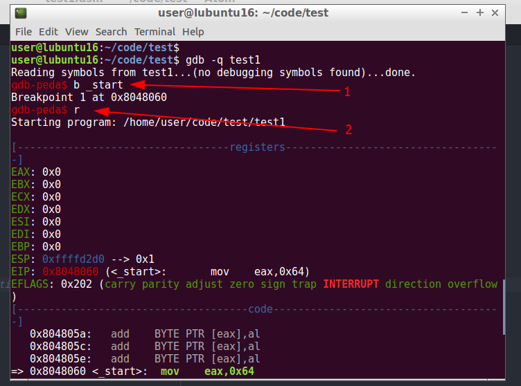
Let’s fisrt set a breakpoint on start by typing: b _start (1)
Then we can run the program by typing: r (2)
Thanks to our peda extension, we see our registers and code:

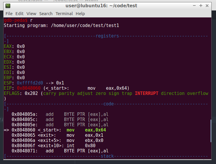
Let’s begin disassembly, we type: disas

Then we use the command si which means step-into to advance to the next instruction.

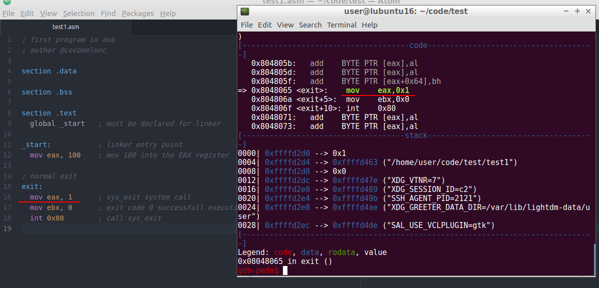
Again, thanks to peda, we see that simply moving 1 into EAX in exit()
If you have not install peda extension, just type: disas:

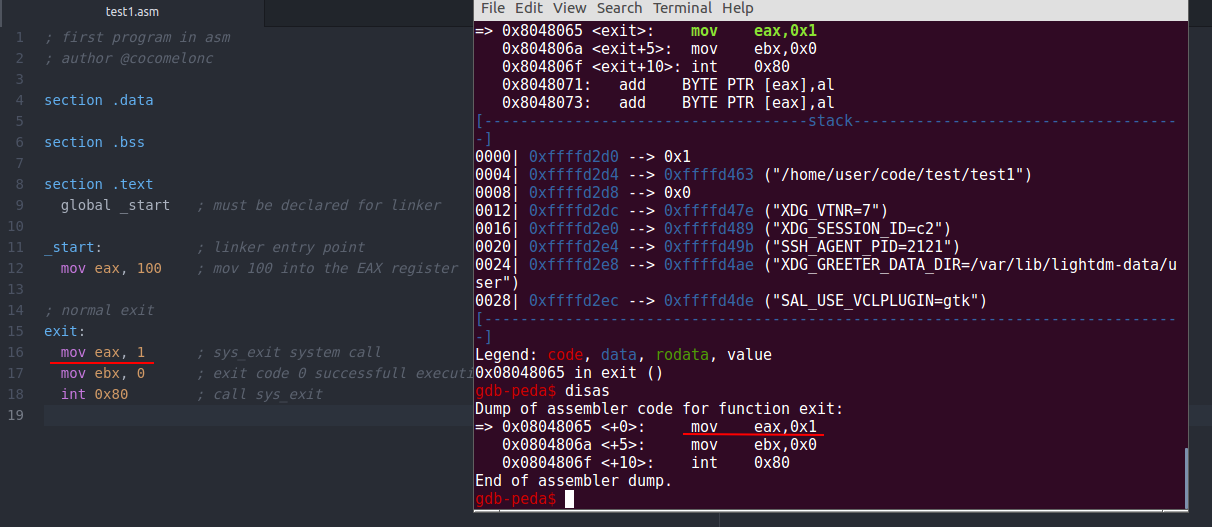
As you can see, it’s the same.

Then, repeat si command (or si and disas if you have not install peda):

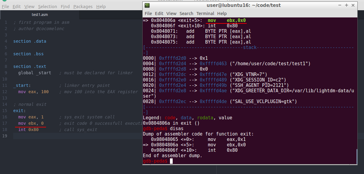
and repeat again si:

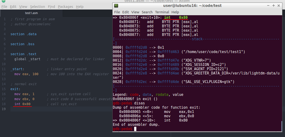
and next step:

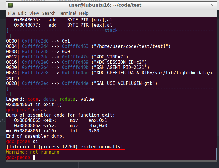
So, as you can see our program exited normally as expected.

With each subsequent post in this series, I will analyze more and more complex examples and try to reverse the more interesting variants of malware. But, of course, I’ll start with simple examples.

Reverse engineering for beginners
CS5138 free course materials
Practical Malware Analysis Book
GDB
pefile
intel 64 and IA-32 arch software developer’s manual

Source code in Github

Thanks for your time and good bye!
PS. All drawings and screenshots are mine